

Integration is one of the most important mathematical tools, especially for numerical simulations. Partial Differential Equations (PDEs) are usually derived from integral balance equations, for example. Once a PDE needs to be solved numerically, integration most often plays an important role, too. This blog post gives an overview of the integration methods available in the COMSOL software and shows you how you can use them.
The Importance of Integrals
COMSOL uses the finite element method, which transforms the governing PDE into an integral equation — the weak form, in other words. Having a closer look at the COMSOL simulation software, you may realize that many boundary conditions are formulated in terms of integrals. A couple of examples of these are Total heat flux or floating potential. Integration also plays a key role in postprocessing, as COMSOL provides many derived values based on integration, like electric energy, flow rate, or total heat flux. Of course, our users can also use integration in COMSOL for their own means, and here you will learn how.
Integration by Means of Derived Values
A general integral has the form
where [t_0,t_1] is a time interval, \Omega is a spatial domain, and F(u) is an arbitrary expression in the dependent variable u. The expression can include derivatives with respect to space and time or any other derived value.
The most convenient way to obtain integrals is to use the “Derived Values” in the Results section of the new ribbon (or the Model Builder if you’re not running Windows®).
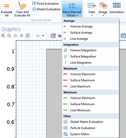
How to add volume, surface, or line integrals as Derived Values.
You can refer to any available solution by choosing the corresponding data set. The Expression field is the integrand and allows for dependent or derived variables. For transient simulations, the spatial integral is evaluated at each time step. Alternatively, the settings window offers Data Series Operations, where Integration can be selected for the time domain. This results in space-time integration.
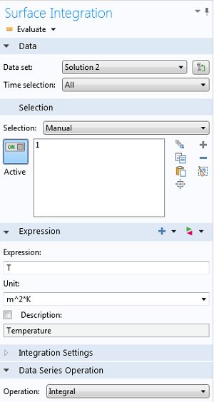
Example of Surface Integration Settings with additional time integration via the Data Series Operation.
The Average is another Derived Value related to integration. It equals an integral, which is divided by the volume, area, or length of the considered domain. The Average Data Series Operation additionally divides by the time horizon. Derived Values are very useful, but because they are only available for postprocessing, they cannot handle every type of integration. That is why COMSOL provides more powerful and flexible integration tools. We demonstrate these methods with an example model below.
Spatial and Temporal Integration for a Heat Transfer Example Model
We introduce a simple heat transfer model, a 2D aluminum unit square in the (x,y)-plane. The upper and right sides are fixed at room temperature (293.15 K) and on the left and lower boundary, a General inward heat flux of 5000W/m^2 is prescribed. A stationary solution and a time-dependent solution after 100 seconds are shown in the following figures.
")
Stationary solution, click image to enlarge.
")
Transient solution after 100 s, click image to enlarge.
Spatial Integration by Means of Component Coupling Operators
Component Coupling Operators are, for example, needed when several integrals are combined in one expression, when integrals are requested during calculation, or in cases where a set of path integrals are required. Component Coupling Operators are defined in the Definitions section of the respective component. At that stage, the operator is not evaluated yet. Only its name and domain selection are fixed.
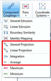
How to add Component Coupling Operators for later use.
For our example, we first want to calculate the spatial integral over the stationary temperature, which is given by
In the COMSOL software, we use an integration operator, which is named intop1 by default.
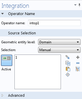
Settings window of the integration operator.
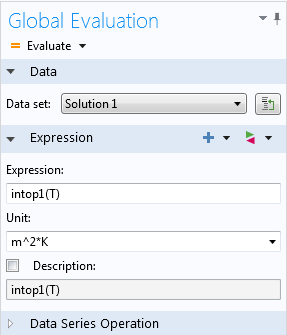
How to evaluate the Integration operator.
In the next step, we demonstrate how an Integration operator can also be used within the model. We could, for example, ask what heating power we need to apply to obtain an average temperature of 303.15 K, which equals an average temperature increase of 10 K compared to room temperature. First, we need to compute the difference between the desired and the actual average temperature. The average is calculated by the integral over T, divided by the integral over the constant function 1, which gives the area of the domain. Fortunately, this type of calculation can easily be done with an Average operator in COMSOL. By default, such an operator is named aveop1. (Note that the average over the domain is the same as the integral for our example. That is because the domain has unit area.) The corresponding difference is given by
Next, we need to find the General heat flux on the left and lower boundary, so that the desired average temperature is satisfied. To this end, we introduce an additional degree of freedom named q_hot and an additional constraint as a global equation. The General inward heat flux is replaced by q_hot.
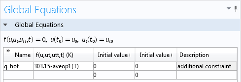
How to add an additional degree of freedom and a global equation, which forces the average temperature to 303.15 K.
Solving this coupled system with a stationary study results in q_{hot}=5881.30 W/m^2. This value has to be prescribed as a General inward heat flux boundary condition to achieve an average temperature of 303.15 K in the whole domain.
Computing the Antiderivative by Means of Integration Coupling
A frequently asked question we receive in Support is: How can one obtain the spatial antiderivative? The following application of integration coupling answers this question. The antiderivative is the counterpart of the derivative, and geometrically, it enables the calculation of arbitrary areas bounded by function graphs. One important application is the calculation of probabilities in statistical analyses. To demonstrate this, we fix y=0 in our example and denote the antiderivative of T(x,0) by u(x). This means that \frac{\partial u}{\partial x}=T(x,0). A representation of the antiderivative is the following integral
where we use \bar x in order to distinguish the integration and the output variable. In contrast to the integrals above, we here have a function as a result, rather than a scalar quantity. We need to include the information that for each \bar x\in[0,1] the corresponding value of u(\bar x) requires an integral to be solved. Fortunately, this is easy to set up in the COMSOL environment and requires only three ingredients, so to speak. First, a logical expression can be used to reformulate the integral as
Second, we need an integration operator that acts on the lower boundary of our example domain. Let’s denote it by intop2. Third, we need to include the distinction of integration and output variable. The notation for this situation is source and destination for x and \bar x, respectively. When using an integration coupling operator, the built-in operator dest is available, which indicates that the corresponding expression does not belong to the integration variable. More precisely, it means \bar x=dest(x) in COMSOL. Putting the logical expression and the dest operator together, results in the expression T*(x<=dest(x)), which is exactly the input expression that we need for intop2. Altogether, we can calculate the antiderivative by intop2(T*(x<=dest(x))), resulting in the following plot in our example:
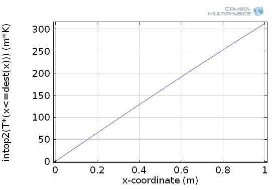
How to plot the antiderivative by Integration coupling, the dest operator, and a logical expression.
COMSOL provides two other integration coupling operators, namely general projection and linear projection. These can be used to obtain a set of path integrals in any direction of the domain. In other words, integration is performed only with respect to one dimension. The result is a function of one dimension less than the domain. For a 2D example the result is a 1D function, which can be evaluated on any boundary. Some more details on how to use these operators are subject to a forthcoming blog post on component couplings.
Spatial Integration by Means of an Additional Physics Interface
The most flexible way of spatial integration is to add an additional PDE interface. Let’s remember the example of the antiderivative and assume that we want to calculate the antiderivative not only for y=0. The task can be formulated in terms of the PDE
with Dirichlet boundary condition u=0 on the left boundary. The easiest interface to implement this equation is the Coefficient Form PDE interface, which only needs the following few settings:
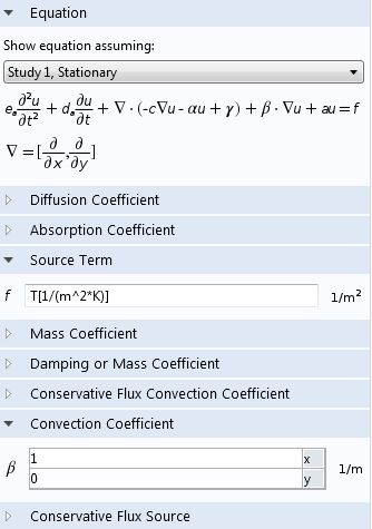
How to use an additional physics interface for spatial integration.
The dependent variable u represents the antiderivative with respect to x and is available during calculation and postprocessing. Besides flexibility, a further advantage of this method is accuracy, because the integral is not obtained as a derived value, but is part of the calculation and internal error estimation.
Temporal Integration by Means of Built-In Operators
We have already mentioned the Data Series Operations, which can be used for time integration. Another very useful method for time integration is provided by the built-in operators timeint and timeavg for time integration or time average, respectively. They are readily available in postprocessing and are used to integrate any time-dependent expression over a specified time interval. In our example we may be interested in the temperature average between 90 seconds and 100 seconds, i.e.:
The following surface plot shows the resulting integral, which is a spatial function in (x,y):
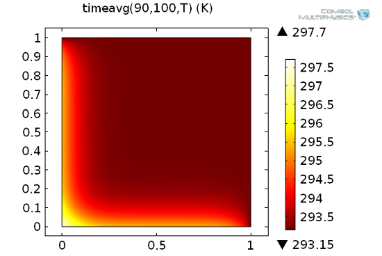
How to use the built-in time integration operator timeavg.
Similar operators are available for integration on spherical objects, namely ballint, circint, diskint, and sphint.
Temporal Integration by Means of Additional Physics Interfaces
If temporal integrals have to be available in the model, you need to define them as additional dependent variables. Similar to the Coefficient Form PDE example shown above, this can be done by adding an ODE interface of the Mathematics branch. Suppose, for example, that at each time step, the model requests the time integral from start until now over the total heat flux magnitude, which measures the accumulated energy. The variable for the total heat flux is automatically calculated by COMSOL and is named ht.tfluxMag. The integral can be calculated as an additional dependent variable with a Distributed ODE, which is a subnode of the Domain ODEs and DAEs interface. The source term of this domain ODE is the integrand, as shown in the following figure.
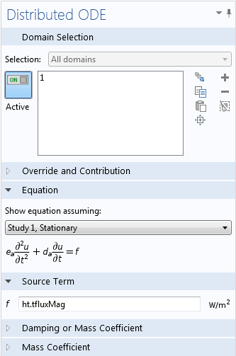
How to use an additional physics interface for temporal integration.
What is the benefit of such a calculation? The integral can be reused in another physics interface, which may be influenced by the accumulated energy in the system. Moreover, it is now available for all kinds of postprocessing, which is more convenient and faster than built-in operators. For an example, check out the Carbon Deposition in Hetereogeneous Catalysis model, where a domain ODE is used to calculate the porosity of a catalyst as a time-dependent field variable in the presence of chemical reactions.
Integration of Analytic Functions and Expressions
So far, we have shown how to integrate solution variables during calculation or in postprocessing. We have not yet covered integrals of analytic functions or expressions. To this end, COMSOL provides the built-in operator integrate(expression, integration variable, lower bound, upper bound).
The expression might be any 1D function, such as sin(x). It is also possible to include additional variables, such as sin(x*y). The second argument specifies over which variable the integral is calculated. For example integrate(sin(x*y),y,0,1) yields a function in x, because integration only eliminates the integration variable y. Note that the operator can also handle analytic functions, which need to be defined in the Definitions node of the current component.
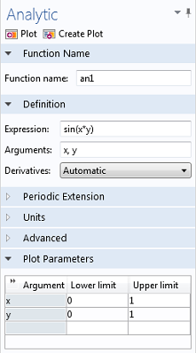
How to add an analytic function.
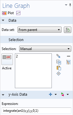
How to integrate over an analytic function.
Further Reading
- Model downloads
- Using Integration coupling operators: Acoustics of a Muffler
- Using global equations for time integration: Process Control Using a PID Controller
- Using global equations to satisfy constraints: Using Global Equations to Satisfy Constraints
- Using domain ODEs for time integration: Capacity Fade of a Li-Ion Battery and Carbon Deposition in Heterogeneous Catalysis
- Knowledge Base entry: Computing Time and Space Integrals


Comments (6)
Jing Huang
February 21, 2014Interesting, but I am wondering how to extend the “Spatial Integration by Means of an Additional Physics Interface” to 2 dimensional?
Malkhaz Meladze
December 1, 2014It is a very interesting topic and well presented too. I gain much from it and I believe many other COMSOL users will benefit from it if the author could make a webinar based on this blog. (I mean webinars are advertised better and have more attention).
Many thanks.
neeraj mishra
May 13, 2016sir my topic is simulation of dielectric elastomer actuator i m using comsol multyphysics 5.0
i m not getting result plz help me .
PFA: this is my base paper
http://www.sciencedirect.com/science/article/pii/S0924424707004335
Mohammad Rahmani
May 9, 2019It is not clear in which version of COMSOL these examples were implemented. It is also difficult to reproduce them as there is no or little information on implementation!
Digvijay Ronge
April 12, 2022For example, if you want to calculate total flow rate (which is pulsating in nature) of fluid coming in/out of a surface, then
Results>Dataset>surface (select the surface)
Results>Dataset>Time integral
Results > Derived values > surface integration >select Dataset ‘Time integral 1’, put expression spf.U and evaluate. You will get total volume of fluid in m^3.
If you want to evaluate flow rate, then instead time integral use time average.
Regards,
Prof. Digvijay Ronge
Yukai Qiao
March 10, 2024Hi, this blog is quite useful for spatial integration. just out of curiosity, is there any example about 3D spatial integration? like a 3D cylinder, instead of calculating the whole volume such as (-10=<z<=10), is there any quicker way to only calculate the middle half (-5=<z<=5)? Sometimes adding another PDE interface or setting two seperate integration coupling operators is more likely to lead to convergency problems during calculation. is there any simple way to do that in postprocessing, from the Derived values??? thx