From your living room to the moons of Saturn, piezoelectric transducers can be found in a wide range of places. These devices are compact, reliable, and self-generating, making them useful for various industries. To optimize the design of these devices, it’s important to account for the phenomena involved, such as electric currents, pressure acoustics, stress-strain, and acoustic-structure interaction. Using the COMSOL® software, engineers can simulate this multiphysics behavior to predict and improve the performance of piezoelectric transducers.
Piezoelectric Transducers: Jumpstarting the Use of Piezoelectricity
Created in 1917, piezoelectric transducers were the first practical use of piezoelectricity, able to transform electricity into sound or sound into electricity. Piezoelectricity was discovered several decades earlier (in the 1880s); however, at the time, there were no real-world applications that electromagnetism, which was more popular and less complex to understand, couldn’t handle. This changed when Paul Langevin and his colleagues created the first piezoelectric transducer. Their device could produce a high-frequency trill underwater and measure the distance between it and another object, advancing submarine detection and sonar research.
Once this discovery was made, piezoelectric transducers became more and more common due to their ability to work as transducers and both produce and detect sound waves. They are now frequently found in anything from medical ultrasound imaging devices to cheap tweeters for laptops. In addition, these transducers have been used to alert landline phone owners when there’s an incoming call as well as to keep precise time in quartz watches. Other uses include:
- Noninvasive medical diagnostics
- Welding plastics
- Ultrasound flowmeters
- Ultrasonic parking sensors
- Nondestructive testing
- Electronic drum pads
- Cleaning for microsystems
- Engine management and fuel injection systems for cars
- Measurement devices (like the penetrometer for the Huygens Probe, which landed on Titan)
- Inkjet droplet actuators
Ultrasonic transducers are often used for medical diagnostic equipment, like the one shown here. Image by Marco Verch. Licensed under CC BY 2.0, via Flickr Creative Commons.
It’s easy to see why these transducers are so popular: They are simple, compact, reliable, and efficient. Even a small amount of electrical energy can generate a lot of sound (or vice versa). What’s more, they have both a high frequency response (making them suitable for ultrasonic technology) as well as a high transient response (meaning they can respond rapidly to changes).
When creating a piezoelectric transducer, it’s important to understand their behavior. This can be a challenge, though, due to the devices’ multiphysics nature, which involves electric fields, structural mechanics, and acoustics. One solution is to use the COMSOL Multiphysics® software and the add-on Acoustics Module…
Modeling the Multiphysics of an Ultrasonic Transducer
The tutorial example featured here is of a simple piezoelectric transducer that could be part of a phased array transducer. A crystal plate made of PZT-5H (a common material for this device) is formed via a series of layers that are separated into periodically repeating rows. The lower surface is grounded, while the upper surface has an applied AC potential of 100 V. The plate itself is rotationally symmetric, so you can model it as 2D axisymmetric geometry for a more efficient simulation.
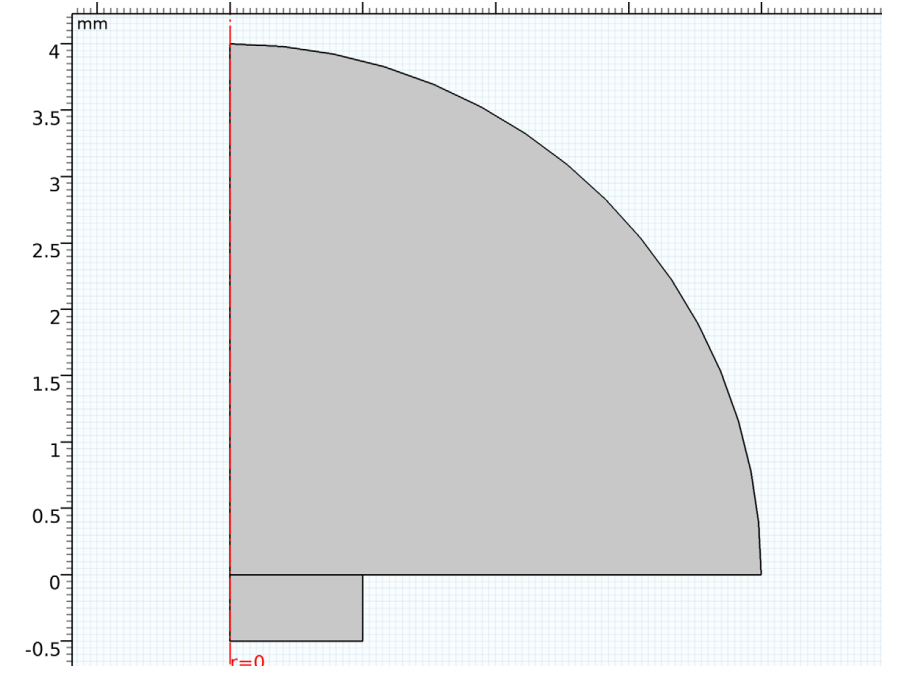
Geometry for the 2D axisymmetric transducer model.
A piezoelectric transducer works via three coupled phenomena:
- A voltage drop is applied over the device (inducing electric currents)
- The alternating current stresses (i.e., excites) the piezoelectric material, which begins to vibrate
- The vibrations generate sound waves that propagate outward
To capture this behavior, you can use the built-in Acoustic-Piezoelectric Interaction, Frequency Domain multiphysics interface. This automatically adds the Electrostatics, Solid Mechanics, and Pressure Acoustics interfaces, which can be easily coupled by applying the Piezoelectric Effect and Acoustic-Structure Boundary multiphysics coupling nodes. Together, these physics interfaces are able to account for the piezoelectric effect as well as how the movement of the solid is transferred into the air surrounding the transducer. Note that in this case, the excitation is 0.2 MHz (10x what humans can hear), making it an ultrasonic transducer.
Evaluating the Performance of the Piezoelectric Transducer
First up for the results, you can visualize the acoustic pressure field in the fluid domain. The image below shows the generated pressure waves in front of the transducer at 0.2 MHz. Notice that the modeling domain only contains a couple of wavelengths. The response outside the domain can be postprocessed using the Exterior Field Calculation feature, as seen below.
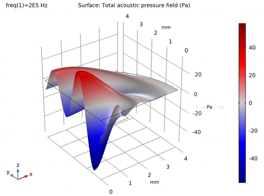
Acoustic pressure distribution in the air surrounding the transducer, visualized here both with colors and a height profile.
In addition, you can evaluate quantities like the sound pressure level (see image below) or intensity in the vicinity of the transducer. This gives an indication of the near-field directivity of the transducer. As expected, the maximum is directly in front of the transducer. The field at any point outside of the computational domain can be visualized using the Exterior Field Calculation feature and the Radiation Pattern plots.
The image below (to the right) shows the far-field radiation pattern (sound pressure level). The far field is mathematically defined as beyond the Rayleigh distance R_0 = S/\lambda, where S is the transducer area and \lambda is the wavelength. For the present example, R_0 = 0.2 mm. At distances beyond R_0, the spatial pattern only scales; that is, it decreases with 6 dB for a distance doubling due to geometric spreading (disregarding dissipation), but does not change its shape.


Left: Sound pressure level distribution in front of the transducer. Right: Radiation pattern depicted in a polar plot. Here, the sound pressure level is for the transducer design.
You can also plot the acoustic pressure or the mechanical stress where the transducer is coupled to the air. These curves are shown in the images below.


Acoustic pressure (left) and the von Mises stress (right) at the air-solid interface for the transducer.
The results above are taken directly from the Piezoelectric Transducer tutorial model. With a few steps, the results can be extended for more frequencies, and the beam width can be computed. First, compute the solution for several frequencies — for example, for 0.2 MHz, 0.3 MHz, and 0.4 MHz — by simply adding those to the Frequencies list in the study. The normalized radiation pattern can be seen below. To normalize to 0 dB in front, plot the expression acpr.efc1.Lp_pext-subst(acpr.efc1.Lp_pext,r,0,z,1[mm]).
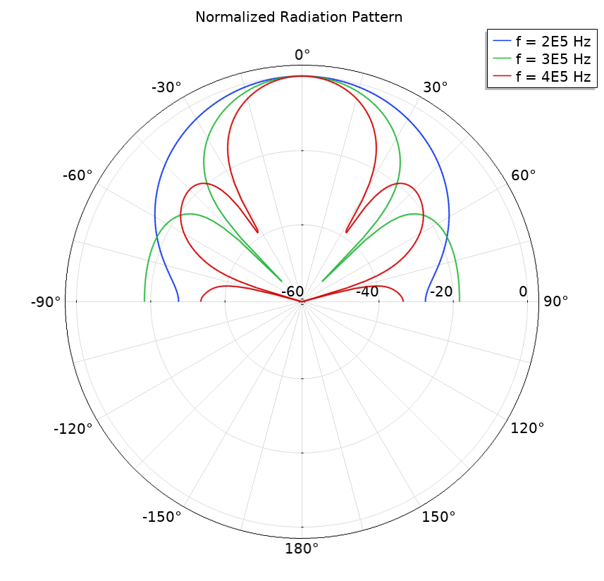
Normalized radiation pattern of the transducer for the selected three frequencies.
To compute the beam width of the radiated field, you can use the built-in functionality in the Radiation Pattern plots. In the plot, simply set the Compute beam width option to On and specify the Level down value. If you enter 3[dB], you will get both the null-to-null beam width as well as the 3-dB down beam width evaluated in a table as a function of frequency. In the table, simply click the Table Graph button to generate a plot. In the image below, the two beam width measurements are depicted as functions of frequency. Here, they are evaluated for 20 frequencies between 0.2 MHz and 0.4 MHz.
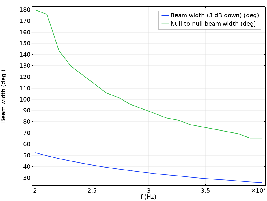
The 3-dB down beam width and the null-to-null beam width of the radiated acoustic pattern plotted as a function of frequency.
With results such as these, engineers can study the performance of a piezoelectric transducer design, using the information to improve it for use in a certain field.
Next Steps
Try modeling a piezoelectric transducer yourself by clicking the button below. This will take you to the Application Gallery, which includes a step-by-step tutorial for this model as well as the MPH file.
Further Resources
- Learn more about modeling piezoelectric transducers on the COMSOL Blog:
- Check out these related tutorials:


Comments (4)
Ramya Ananda Natarajan
August 13, 2019I want to make the sound propagate through a metal (solid) this model works for air and liquid. What changes do I need to make for the sound to propagate through a solid?
Mads Herring Jensen
August 13, 2019 COMSOL EmployeeHi Ramyan
To make the sound propagate through a solid you have to replace the Pressure Acoustics, Frequency Domain physics interface with Solid Mechanics. The Solid Mechanics interface uses a full formulation of the governing equations in solids so it also models elastic waves!
Best regards
Mads
Mads Herring Jensen
August 13, 2019 COMSOL EmployeeHi Ramya
To model a metal you have to replace the Pressure Acoustics, Frequency Domain physics interface with Solid Mechanics. The Solid Mechanics interface uses a full formulation of the governing equations in solids so it also models elastic waves in the frequency domain!
Best regards
Mads
Ashley Poole
August 3, 2020Im trying to simulate a shear rate induced by an ultrasonic transducer, what physics would you recommend?