Using Symmetry to Reduce Model Size
One of the ways you can simplify and reduce the size of a finite element model is by using any symmetries present in your model. Whether you are building the geometry natively in COMSOL Multiphysics® or importing a design from an external file, there are modeling strategies as well as features in the software that you can use to take advantage of such symmetries. In this article, we will explain how you can take advantage of symmetry in your simulation to reduce its size and discuss the functionality in the software that enables you to easily do so.
Advantages
Reducing the size of your model is advantageous because of the amount of computational time and memory that can be saved when solving the equations for your model. These savings can be significant when working with large models and multiphysics models. It is also beneficial regardless of the phase of model development that you are currently working in. If you are starting a model from scratch, by using a reduced, simplified version of your design, you can take less time to set up and build your model and reach results. From there, you can continue to expand the scope of your simulation and increase complexity.
 The complete geometry of a circular heat sink with 8 fins in 3D.
 Geometry of the top half of a heat sink.
 The cross-sectional geometry of the top half of a heat sink in 2D.
If you are working with a geometry that has already been fully built, reducing its size can help you reach solutions for the model equations more quickly. You can then perform postprocessing in order to visualize the solution for the entire model geometry. Additionally, reducing your model size enables you to catch and resolve any errors in your model setup more quickly.
Symmetry and Geometry Simplification
By using the symmetries in a model, you can reduce its size by half or more, making this an efficient method for solving large models. This applies to cases where both the geometry and modeling assumptions include symmetries. It can also be the case that neglecting, or omitting, some geometric or other modeling features will allow for additional symmetry to be used. Some common types of symmetries are axial symmetry as well as symmetric and antisymmetric planes and lines. Modeling in axial symmetry in particular is very efficient, but often involves assuming that some modeling features can be neglected.
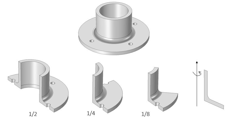
The geometry for a flange. In lieu of modeling the entire flange, the axisymmetric nature of the design can be used to reduce its model size by half, a quarter, an eighth, and down to a cross section. Reducing to axial symmetry is valid if it can be assumed that the bolt holes do not significantly affect the solution.
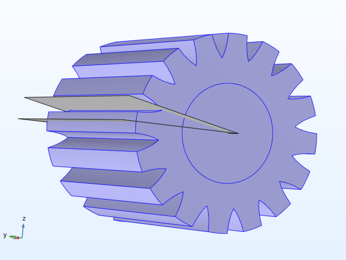
An example geometry that exhibits cyclic symmetry. The symmetry planes are indicated by two gray work planes.
Axial Symmetry
Axial symmetry is common for cylindrical and similar 3D geometries. If the geometry is axisymmetric, there are variations in the radial (r) and vertical (z) direction only, i.e., not in the angular ( ) direction. You can then solve a 2D problem in the rz-plane instead of the full 3D model, which can save significant computational memory and time. Most physics interfaces in COMSOL Multiphysics® are available in axisymmetric versions and take the axial symmetry into account. In addition, several interfaces allow for an assumed form of azimuthal variation, including:
- Fluid Flow, as in the Swirl Flow Around a Rotating Disk tutorial model
- Structural Mechanics, as in the Axisymmetric Twist and Bending tutorial model
- Wave Electromagnetics, as in the Axisymmetric Cavity Resonator tutorial model
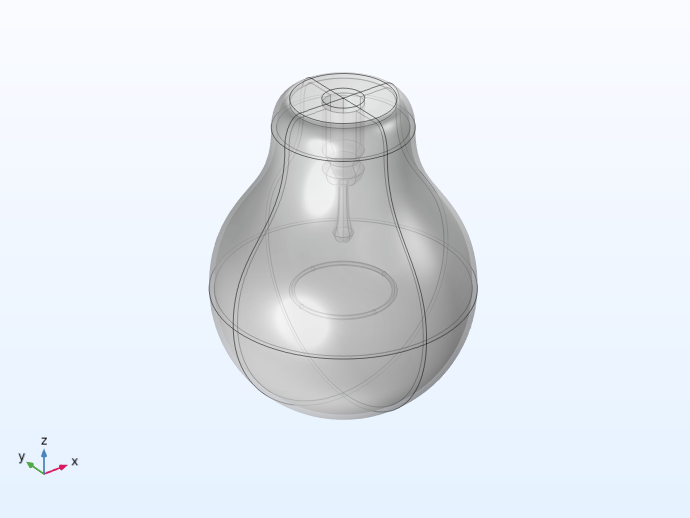 A 3D model of a light bulb.
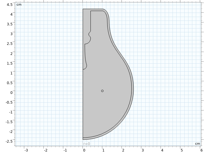 Half of a 2D light bulb as shown as an axisymmetric cross section.
Symmetry Planes and Lines
Symmetry planes and lines are common in both 2D and 3D models. Symmetry means that a model is identical on either side of a dividing line or plane. For a scalar field, the normal flux is zero across the symmetry line. In structural mechanics, the symmetry conditions are different. Many physics interfaces have symmetry conditions directly available as features.
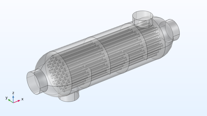 A complete, transparent model of a shell-and-tube heat exchanger in 3D.
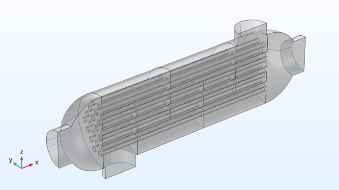 Half of a transparent shell-and-tube heat exchanger model in 3D.
To take advantage of symmetry planes and symmetry lines, all of the geometry, material properties, and boundary conditions must be symmetric, and any loads or sources must be symmetric or antisymmetric. You can then build a model of the symmetric portion, which can be half, a quarter, or an eighth of the full geometry, and apply the appropriate symmetry or antisymmetry boundary conditions.
Antisymmetry Planes and Lines
Antisymmetry planes and lines means that the loading of a model is oppositely balanced on either side of a dividing line or plane. For a scalar field, the dependent variable is 0 along the antisymmetry plane or line. Structural mechanics applications have other antisymmetry conditions. Many physics interfaces have symmetry conditions directly available as features.
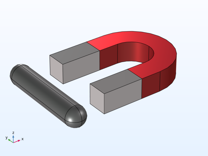 A complete red and gray magnet model in 3D.
 One-fourth of a red and gray magnet model in 3D.
Functionality for Utilizing Symmetry
Partition Operations
Partition Operations enable you to split up any geometric entity, whether it be objects, domains, boundaries, or edges. You can divide up your geometry using another geometric object or a work plane, and then use the Delete operation to remove the unnecessary entities.
Cross Section Operation
The Cross Section operation enables you to go from modeling a solid to a plane. A work plane is used in combination with this operation to extract a cross section from a 3D geometry, which can be used within a 2D or 2D axisymmetric model component.
Projection Operation
The Projection operation enables you to project 3D objects in order to create 2D curves. The geometry can be projected onto a work plane in a 3D model component or in a 2D model component. This is useful for complex geometries, as you can specify what 3D entities (objects, domains, boundaries, edges, points) you want to project into 2D. This is an alternative to having a work plane cut through the geometry and the entire geometric object, such as what is done for the Cross Section operation.
Physics Features and Boundary Conditions
As noted earlier, there are a plethora of physics interfaces that are available in 2D and 2D axisymmetric versions. Additionally, there are many physics interfaces that have different types of symmetry conditions available as physics feature nodes. These include Symmetry, Symmetry Plane, and Antisymmetry boundary conditions, among other types of symmetry boundary conditions (e.g., Sector Symmetry), which enable you to specify the symmetry planes or lines of symmetry in your model.
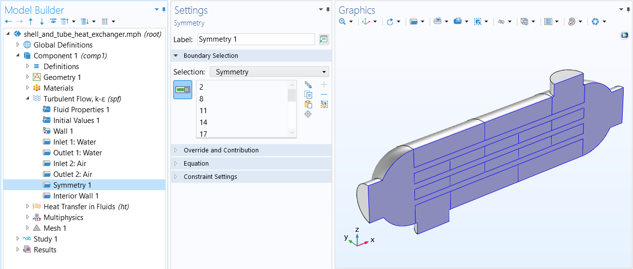 The Symmetry boundary condition that is used in the Shell-and-Tube Heat Exchanger tutorial model.
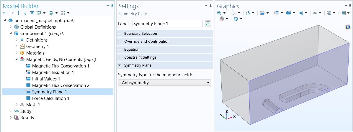 The Symmetry Plane boundary condition that is used in the Permanent Magnet tutorial model, where we specify the antisymmetry of the magnetic field. There are also several other ways you can use symmetry to simplify magnetic field modeling.
Possible Pitfalls for Structural Mechanics Models
There are some cases where the results of structural mechanics models are not purely symmetric, even though the problem may appear so at first. You should note such cases, which include the following:
- Eigenfrequencies in symmetric structures can be both symmetric and antisymmetric. You need to do two studies of half the geometry, one with each set of boundary conditions in order to capture all the eigenfrequencies. If there are multiple symmetries (like modeling a quarter of a structure) all permutations of boundary conditions must be considered.
- In linearized buckling analysis, the lowest buckling mode of a symmetric structure can be either symmetric or antisymmetric (in the same way as the abovementioned point).
- Axial symmetry can only be used to find axially symmetric eigenmodes in the case of eigenvalue analysis (eigenfrequency or buckling).
- Antisymmetric boundary conditions are generally not compatible with geometrically nonlinear analysis of solids since the constraint will remove some strain terms necessary for describing a finite rotation at the antisymmetry section.
Further Learning
There are several blog posts that discuss taking advantage of the symmetries in a model for different application areas. There are also several tutorial models available in the Application Libraries that show different implementations of taking advantage of the symmetries in a geometry. From these you can explore, learn from, and understand the logic that was used for reducing the computational domain as a result of any symmetries. A small sample of the available examples are listed below.
- Vibrations of an Impeller
- Type of symmetry: Cyclic
- Model implementation: Cyclic symmetry boundary conditions (Periodic Condition) applied on two sector boundaries to model 1/8 of geometry
- Heat Transfer by Free Convection
- Type of symmetry: Plane
- Model implementation: Symmetry planes used to model thin domains
- Thermal Contact Resistance Between an Electronic Package and a Heat Sink
- Type of symmetry: Cyclic
- Model implementation: Plane and cyclic symmetry used to model 1/16 of geometry
- Microwave Oven
- Type of symmetry: Plane
- Model implementation: Reflection symmetry used to model 1/2 of geometry
- Muffler with Perforates
- Type of symmetry: Plane
- Model implementation: Symmetry boundary condition applied to model the upper half of geometry
Submit feedback about this page or contact support here.