Setting Up and Solving Electromagnetic Heating Problems
Many multiphysics models involve physics that have different characteristic time scales. One of the most common cases is electrothermal heating. For example, consider a heater connected to the electrical grid. The current in the device is varying sinusoidally at 60 Hz, but you may want to simulate the heating over several minutes or longer, and the magnitude of the current might be modulated during that time period. It can also be that the excitation is periodic but nonsinusoidal. In addition, the material properties are temperature dependent, thus the electromagnetic field solution will vary as the system heats up. Solving for both the transient electromagnetic fields and the temperature fields as the part heats up would be very time consuming and is usually unnecessary. A variety of different solution approaches exist that can solve these types of problems efficiently, depending on the type of problem being considered.
Overview and Analysis Categories
The temperature of a system can be solved for as varying in time or in the stationary limit. It is appropriate to model solely the stationary limit if the variations in time are not of interest. The stationary limit is also usually the worst-case scenario, when the temperatures are the most extreme.
The thermal materials properties (thermal conductivity, density, and specific heat) all depend on temperature, although they are sometimes approximated as constant. Convective and radiative heat transfer both depend on the magnitude of temperature differences. For these reasons, the thermal problem is usually nonlinear.
Many of the existing materials in the Materials Library already have the temperature dependency of the materials properties defined. If you are manually defining a material, make sure to define temperature as an input to the material model, as demonstrated here: Creating a New Material. Then define expressions for the temperature-dependent properties, as shown here: Material Functions.
When modeling an electrical system, the time-dependent variation of the excitation signal can be categorized as:
- Stationary: The excitation is not varying in time, also called DC or steady state.
- Time dependent: The excitation varies arbitrarily in time.
- Frequency domain: The excitation is varying sinusoidally in time at a single frequency. This excitation can be of any frequency. At lower frequencies, it is often referred to as an AC analysis; at higher frequencies, the fields will be wave-like and radiating.
- Modulated: The excitation changes in magnitude over time at a rate that is very different from other electrical time scales.
- Periodic: The excitation varies periodically but nonsinusoidally. Periodic signals are composed of a sum of different frequency-domain signals.
The electrical response of the system to these types of excitations is either:
- Linear: This means that all of the electrical material properties are treated as constants. Although this is a simplifying approximation, it is often a good starting point.
- Indirectly nonlinear: The electrical material properties can vary, but are not varying directly based on the electric or magnetic fields. This is the most common case and typically involves a material with electric conductivity that is a function of temperature.
- Directly nonlinear: The electrical material properties are directly dependent on the electric or magnetic fields.
If the electrical material properties and the electrical boundary conditions do not depend on temperature, then it is possible to treat the problem as one-way coupled, meaning that the electrical problem can be solved first, and the results can be passed to the thermal problem.
If the electrical material properties, such as the electric conductivity, depend on temperature, then the model has to modeled as bidirectionally coupled, meaning that the electrical and thermal problem have to be solved together. This is more computationally expensive than solving a one-way coupled problem.
When solving for a frequency-domain excitation, it is often reasonable to assume that the electrical material properties are approximately constant over at least several periods of the excitation, even if the electrical properties are dependent on temperature. That is, the variation in the temperature, and hence the electrical material properties, varies relatively slowly compared to the period of the electrical excitation. Thus, the variation in the heat loads over one period does not need to be considered, and the cycle-averaged losses, rather than the instantaneous losses, are used in the thermal model. In this case, it is possible to solve as a bidirectionally coupled problem, with the electrical model being solved in the frequency domain. The electrical model will still get recomputed when the temperature change is great enough to affect the electrical material properties.
If the electrical response is directly nonlinear, then this usually needs to be solved as a time-dependent model, with both the electromagnetic and thermal physics being solved in the time domain. There are some specific cases that can be solved in the frequency domain, such as the modeling of nonlinear magnetic materials. If such a simplification, or a similar one, can be used, it will save significant computational cost.
Fundamentals of Setting Up a Model
A minimal electromagnetic heating model must consist of the following: one physics interface that solves for the temperature fields; one physics interface that solves for the electric, and possibly magnetic, losses; and a feature that couples the two physics interfaces together. For an introduction to setting up such a model in the context of electric currents, see Introduction to Electro-Thermal-Mechanical Modeling. For an introduction to such models in the context of low-frequency electromagnetic problems involving induction heating, see Modeling the Heating of Moving Parts in Coils. For an introduction to modeling in the wave electromagnetic regime, see Simulating RF Heating in COMSOL Multiphysics.
The figure below shows the features for an electromagnetic heating model.
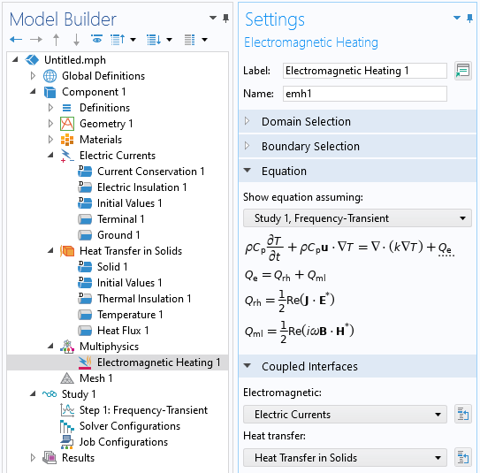
Setup of a typical electromagnetic heating model. The Multiphysics branch with the Electromagnetic Heating multiphysics coupling feature informs the software which physics interfaces are coupled.
An Electric Currents physics interface includes a set of boundary conditions that lead to current flow in the materials. The Heat Transfer in Solids physics interface includes a set of boundary conditions such that the heat generated from the electrical dissipation can leave the modeling domain. The Multiphysics > Electromagnetic Heating feature informs the software that the two physics are coupled. The feature will couple all the losses on domains and boundaries and let the software know that certain specialized study types can be used. The list of these studies is shown below.
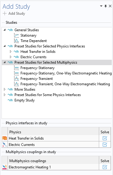
Available study types to choose from when an Electromagnetic Heating multiphysics coupling feature is present and being solved for.
There are several default studies available:
- Stationary: This performs a stationary electrical and stationary thermal analysis and assumes that the model is bidirectionally coupled.
- Time Dependent: This performs a time-dependent electrical and time-dependent thermal analysis and assumes that the model is bidirectionally coupled.
- Frequency-Stationary: This performs a bidirectionally coupled frequency-domain electrical analysis and a stationary thermal analysis.
- Frequency-Stationary, One-Way Electromagnetic Heating: This first performs a frequency-domain electrical analysis and then a stationary thermal analysis. The study consists of two sequential steps.
- Frequency-Transient: This performs a bidirectionally coupled frequency-domain electrical analysis and a time-dependent thermal analysis.
- Frequency-Transient, One-Way Electromagnetic Heating: This first performs a frequency-domain electrical analysis and then a time-dependent thermal analysis. The study consists of two sequential steps.
When these studies are added to the model, they will automatically define the appropriate study steps. Other cases may require manual setup and understanding how the dissipations computed by the electromagnetic model are coupled with the thermal model.
Coupling the Electromagnetic Model with the Thermal Model
The Electromagnetic Heating feature within the Multiphysics branch will automatically couple all thermal losses computed by the selected electromagnetics interface and apply it as a heat load. It works for all cases involving any of the default study types. For other case it will sometimes be necessary to manually define the coupling between the electromagnetic and the thermal model.
The heat dissipated within domains can be manually coupled via the Heat Source domain feature, as shown in the image below. This feature should be applied to all domains where the electromagnetic problem is being solved. To reproduce the functionality of the Electromagnetic Heating feature, enter the software-defined expression for the domain losses computed by the electromagnetic physics interface being solved. The list of such software-defined expressions can be found here: Viewing and Accessing the Equations and Variables for Physics Feature Nodes.
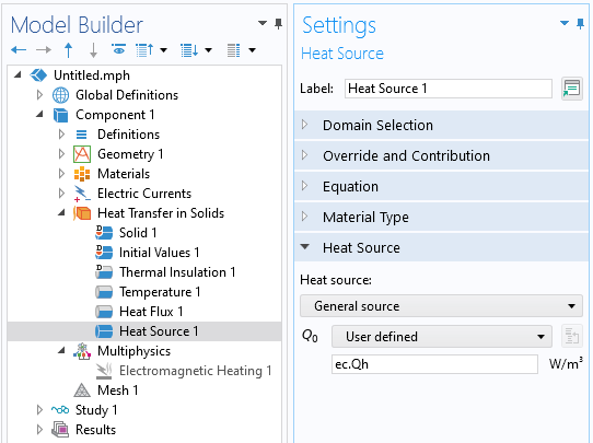
The Heat Source domain feature couples the losses computed from one physics interface with the thermal model. Note that the Electromagnetic Heating feature in the Multiphysics branch is disabled.
If the physics interface solving for the electromagnetic fields additionally computes losses on boundaries, then it is also necessary to introduce a Boundary Heat Source feature where you enter the software-defined expression for the boundary losses. This feature should only be applied on boundaries where surface losses are being computed.
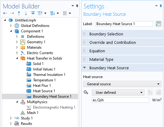
The Boundary Heat Source feature couples the losses computed from one physics interface with the thermal model. Note that the Electromagnetic Heating feature in the Multiphysics branch is disabled.
This set of features reproduces the Multiphysics > Electromagnetic Heating feature, so make sure to use one approach or the other but not both, as that would result in the losses being counted twice.
Understanding the Setup of One-Way Coupled Models
There are two approaches to setting up a one-way coupled model. It is possible to solve the electromagnetic model in one study, with one step, and then in a separate study solve the thermal model with one step. It is also possible to use one study with two study steps, the first solving the electromagnetic model and the second step solving the thermal model.
An example of using a single study with two steps is shown in the images below, which show what happens when the default Frequency-Transient One-Way Electromagnetic Heating study type is added. When the study is solved this way, with one physics being solved after another within a single study, the results from the first study step will automatically propagate to the subsequent step and will be used throughout the second step. Even though it is possible to generate a set of results within the first step — for example, by entering a range of frequencies within the Frequency Domain study type — the first study step should be set up to only generate a single result.
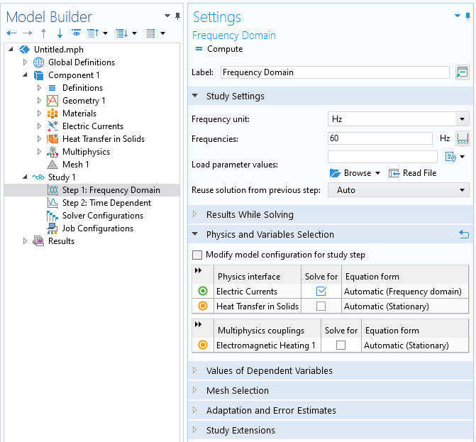
A one-way coupled approach using a single study. The study contains multiple steps, where the first step solves the electromagnetic model. This set should only generate a single result.
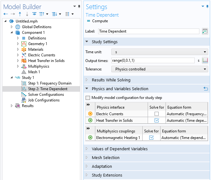
A one-way coupled approach using a single study. The second study step will automatically use the results from the first step.
It is also possible to solve the two physics in separate studies. The first study solves the electromagnetic model and can generate a set of results from a frequency sweep, a parametric sweep, or even a time-dependent study. These results can then be passed to the second study, which solves the thermal model.
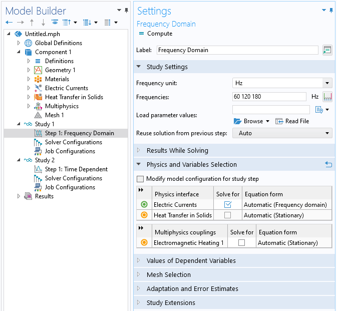
A one-way coupled approach using two studies. The first study solves the electromagnetic model, and a set of results can be generated at once from a frequency sweep, for example.
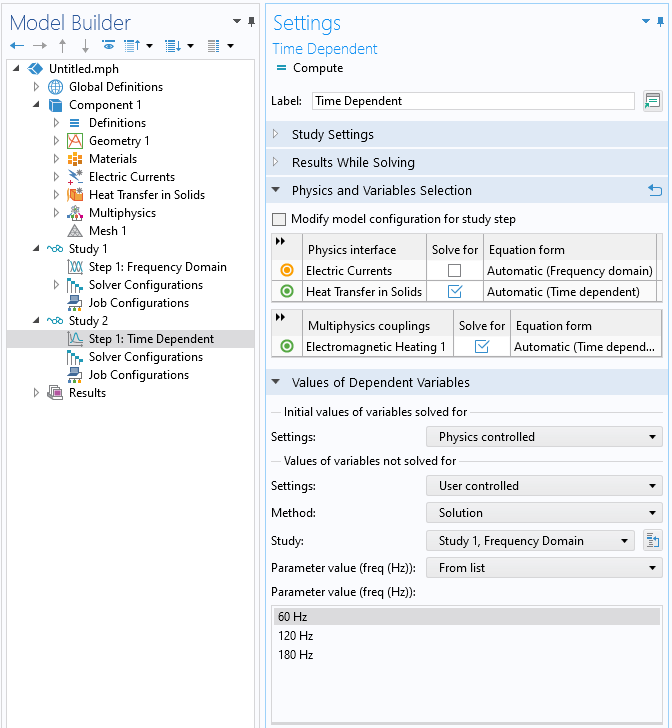
A one-way coupled approach using two studies. The second study solves the thermal model, and the Values of Dependent Variables settings are used to specify which results from the first study are to be used.
Use the Values of Dependent Variables settings within the study step that solves for the thermal problem. This includes a Values of variables not solved for setting and allows for selecting any result from any other previously computed study to be used. When the first study contains a sweep over frequency or a model parameter, only one of these cases can be used within the second study.
It is also possible to manually specify which data or combination of data is passed from one study to another via the withsol() operator. See Examples of the withsol Operator for a general introduction to this functionality. This has to be used with a manual definition of the electromagnetic heat sources, rather than using the Electromagnetic Heating feature. For example, an expression of the form
withsol('sol1',ec.Qh,setval(freq,60))+ withsol('sol1',ec.Qh,setval(freq,180))
will take the sum of the heating at two different frequencies from one study and use it within the second study. When this approach is used, the Electromagnetic Heating feature should be disabled.
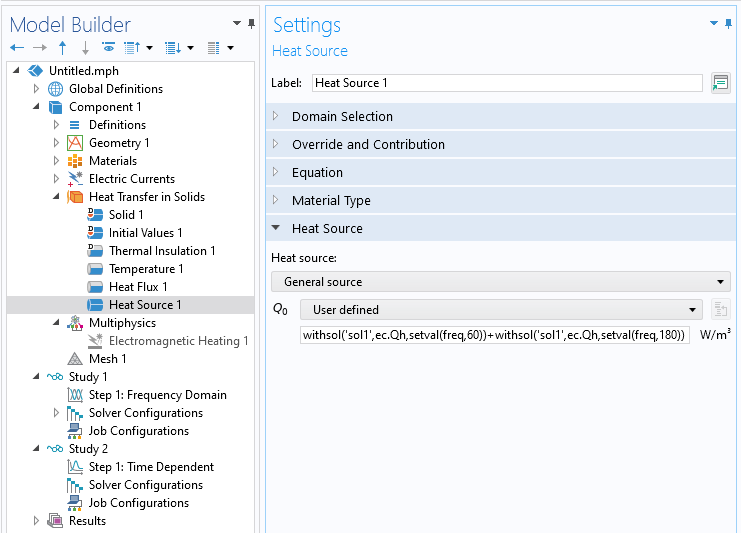
A one-way coupled approach using two studies. The first study solves for a range of frequencies. The second study solves the thermal model, and the expression within the Heat Source feature refers to a combination of results from the first study. Since the heat source is manually defined, the Electromagnetic Heating feature is disabled.
Modifying the Form of the Governing Equation for Bidirectionally Coupled Models
The default behavior of the software is to let the study step control the temporal form of the governing equation. For example, the Electric Currents interface can be used in conjunction with Stationary, Time Dependent, or Frequency Domain study steps. The choice of study step thus determines the equation being solved. It can be desirable to override this for bidirectionally coupled models.
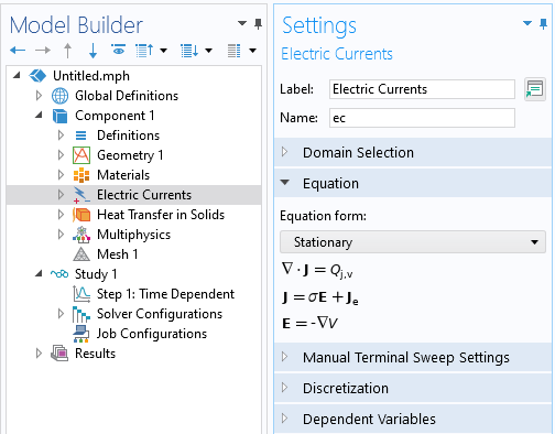
The Equation form setting can be used to manually change the form of the governing equation to be different from the study type. With the settings as shown, the model will solve a bidirectionally coupled model with the electromagnetic fields solved in the stationary form, along with the transient temperature variation.
To solve for the transient temperature variation in a model where the electrical excitation is steady state, use the Time Dependent study type but manually specify that the Electric Currents be solved in the stationary form. This is done via the Equation setting within the physics interface, as shown in the image above. Even though the study uses a Time Dependent study step, only the thermal model will be solved in the time domain; the Electric Currents interface will be solved as a stationary equation at each time step taken by the solver. The assumption of this approach is that the electric fields respond instantaneously to any changes in the materials properties and that any dynamics of the electrical response are negligible. This assumption simplifies the form of the equation being solved by the physics interface.
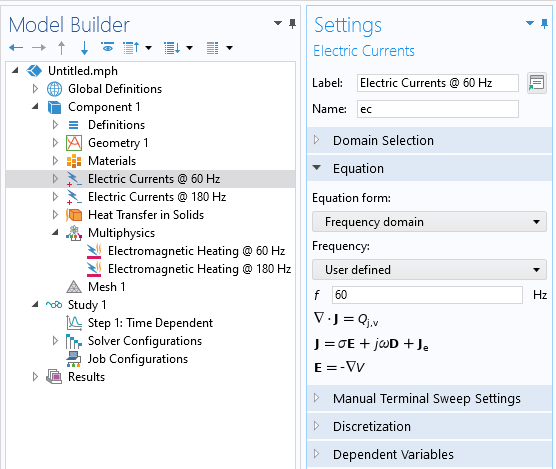
Manually setting the excitation frequency via the Equation settings for a bidirectionally coupled model solving for transient temperature variations and involving multiple excitation frequencies.
It is also possible to manually specify the physics interface while solving in the frequency domain via the Equation setting. This is useful when you want to set up a bidirectionally coupled model that considers heating due to a sum of different excitation frequencies. Use one physics interface for each frequency being considered, as shown in the image above. Additionally, one Electromagnetic Heating feature is needed for each physics interface representing a different frequency, such that the cycle-averaged contributions from each different frequency are applied as heat loads. A Stationary or Time Dependent study can be used in conjunction with this, and the electromagnetic fields will be recomputed at each solver iteration.
Modeling of Modulated Signals in Bidirectionally Coupled Models
Modeling of modulated electrical signals is only in the context of transient thermal analysis. There are two kinds of modulated signals: slow-varying and discretely varying. This categorization applies to modulation of both DC and AC signals, as shown in the figure below.
Slow-varying means that the characteristic time of the modulation is much longer than the characteristic electrical timespan of the system. That is, any leading or lagging due to the system capacitance or inductance will happen much faster than the modulation. Additionally, the excitation frequency is much faster than the modulation.
A discretely varying modulation happens much more quickly than the electrical timespan or applied signal. Such a fast change in the applied signal will often lead to a complicated oscillatory response over a relatively very short period, governed by the system capacitance and inductance. It is often sufficient to ignore this and instead approximate the electric fields as changing instantaneously.
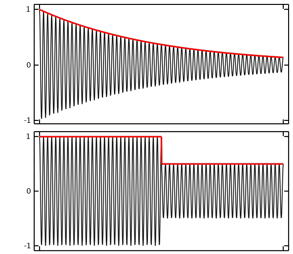
The two types of modulations. Top: slowly varying modulation of a DC (red) and an AC (black) signal. Bottom: discrete modulation of DC (red) and AC (black) signals.
Slow-varying modulation is addressed by making the expression for the excitation magnitude a function of time. For example, to set up an applied current that exponentially decays in magnitude over the span of hours, use an expression in terms of the time variable
10[A]*exp(-t/1[h]).
When solving with such a slow excitation, it is appropriate to manually modify the form of the governing equation such that the electromagnetic problem can be treated as a stationary model. This same expression is also valid in the frequency domain, where AC variation is implicitly assumed. So when the above expression is used in a bidirectional Frequency-Transient study, it implies a sinusoidal excitation at the specified frequency that is modulated by the above expression.
Discretely varying modulation is modeled via the Events interface, which specifies for the solver the times at which the signal changes magnitude. The two components to this interface are a Discrete States variable and an Explicit Event. A Discrete States variable is used to modulate the magnitude of the signal. The Explicit Event is used to specify the possibly periodic times at which the signal magnitude changes as well as the change in the variables controlling the excitation. Both DC and AC signals can be modified in this way.
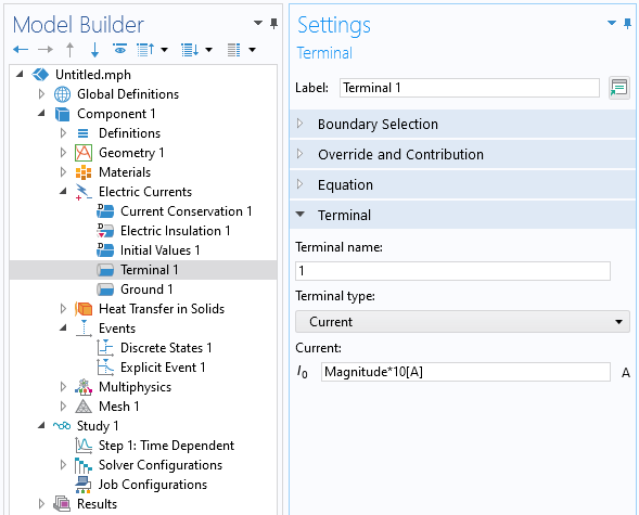
The magnitude of the applied current is controlled via a Discrete State variable.
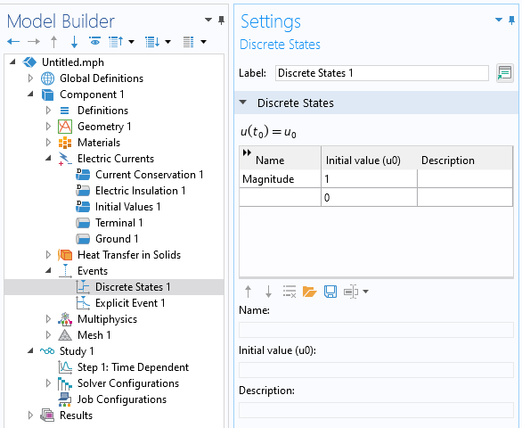
The Discrete States feature defines the initial condition of the variables.
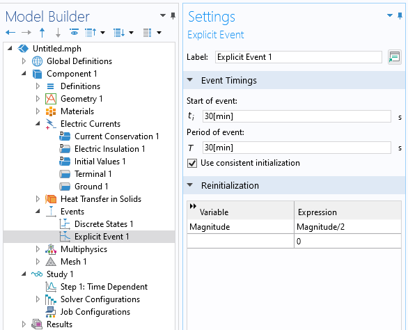
The Explicit Event feature specifies when and how discrete state variables are updated.
In addition to explicit modulation of the applied signal magnitude, it is also possible to set up an implicit modulation based on a threshold condition. Typically, this is done based on the temperature field. For example, an electrical heater will turn on once the temperature drops below a threshold, and then turn off once the temperature rises above a different threshold. This type of control is implemented via the Implicit Events interface, which is covered in Solving Models with Step Changes to Loads in Time.
Modeling of Periodic Signals in Bidirectionally Coupled Models
Periodic signals, such as a triangular waveform, repeat in time but are not sinusoidal. If it can be assumed that the electrical material properties remain approximately constant over one period, then such signals can be approximated via the Fourier transform as the sum of a set of frequency-domain signals. For instance, the Fourier series of a triangular wave with fundamental angular frequency  is
is

So, a triangular wave can be approximated by taking a finite sum of the odd harmonics of the fundamental frequency, each of which will contribute to the heating. For the triangular waveform, it is often sufficient to only consider the first and third harmonics.
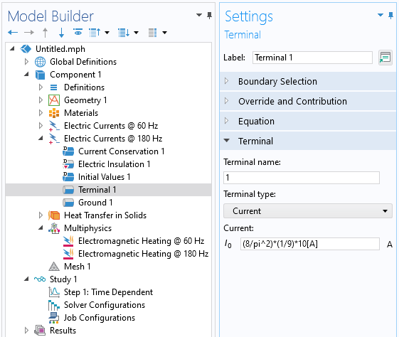
For bidirectionally coupled models excited with periodic signals, use one physics interface per harmonic to resolve the signal, and use the Fourier coefficient for each harmonic.
Each harmonic needs to be solved simultaneously with the thermal model, so add one physics interface per harmonic and manually specify the equation form to be in the frequency domain. Modify the excitations based on the Fourier coefficients of the applied periodic signal. For the triangular waveform case, the Fourier coefficients are known, but for signals that do not have analytic expressions, instead use the Time to Frequency FFT study type to compute the coefficients (as described here) and use the withsol operator to take these values from the FFT results. It is also important to study how many harmonics are sufficient to capture the heating (as described here) since several more harmonics might be needed depending on the waveform.
Submit feedback about this page or contact support here.