
For many mechanical contact problems, stick-slip friction transition is an important point of analysis. When present, this phenomenon influences the stresses, strains, and deformations near the contact area between the two bodies. In version 5.3 of the COMSOL Multiphysics® software, we have the tools necessary to handle this type of mechanical contact problem and validate the results. With a better understanding of stick-slip friction transition and its subsequent effects, we can improve the safety and energy efficiency of relative systems.
The Stick-Slip Phenomenon in Mechanical Contact Problems
On any given day, we can hear the noises from car tires or trains as they come to a stop. While the sounds themselves are familiar, the phenomenon behind them might not be.

The stick-slip phenomenon is present in many applications, such as when a train comes to a stop. Image by DozoDomo. Licensed under CC BY-SA 2.0, via Flickr Creative Commons.
Stick-slip — common in mechanical contact applications — describes the motion that occurs when two surfaces alternate between sticking to one another and sliding over each other. As this motion occurs, corresponding changes take place in the force of the friction. Collectively, these interactions can impact the stresses, strains, and deformations that occur close to where the two bodies are in contact. This in turn influences the efficiency of the system as well as its safety.
There is a new tutorial available in the Application Gallery that handles a transient contact problem involving stick-slip friction transition. Let’s have a look at the setup of this model and the results that it produces.
Note: This example is currently available via the Application Library update.
Analyzing a Transient Contact Problem in COMSOL Multiphysics®
For this example, our model geometry consists of a halfpipe and a section cut from a hollow pipe. The halfpipe features a transition length of 50 cm and a radius of about 1 m. Meanwhile, the pipe has a thickness of 2 cm and a radius of 15 cm.
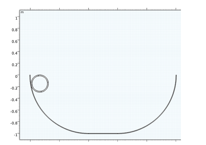
The model geometry.
Subjected to a gravity load, the pipe is released at the top of the halfpipe with its centroid 75 cm above the horizontal plane. These two bodies remain in contact with one another at all times. Depending on the velocity of the pipe and its location in the halfpipe, the motion of the pipe fluctuates between sliding and rolling. We define the friction coefficient as a function of the slip velocity via the exponential dynamic Coulomb friction model.
For this simulation study, the values of interest are pipe displacement and energy balance — the latter of which is used to verify the accuracy of the results. The solution is computed for a time of four seconds.
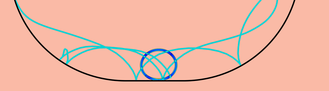
The plot below depicts the von Mises stress distribution in the pipe at the final step and the trajectory of a point located on its outer surface. It is clear that the pipe deforms due to gravity and that the trajectory path transitions between stages of stick and slip friction. In the stick stage, the trajectory is smoothly parabolic in correlation with the rotation of the pipe. In the slip stage, the trajectory is slightly more elongated. From the following animation, we can see the evolution of the pipe’s motion over time.

The stress distribution in the pipe and the point trajectory.
The motion of the pipe over four seconds.
Let’s now check the energy balance. As expected, the potential energy (green) becomes lower as the kinetic energy (blue) rises. Because of frictional dissipation energy (red), the pipe is never able to reach its initial height on the halfpipe. The majority of the energy is lost due to the friction that occurs when the pipe arrives at the steeper slope area of the halfpipe. After two seconds, the pipe stays in the region with the lower slope and rolls rather than slides. Because of the pipe’s deformable behavior, some of the total energy (pink) is stored as elastic strain energy (light blue). In the plot below on the right, we can visualize the friction coefficient as a function of time. As the results indicate, the exponential dynamic Coulomb friction coefficient causes the friction to drop exponentially as the slip velocity increases.
Energy balance versus time.

The friction coefficient as a function of time.
Addressing Stick-Slip Friction Transition in Transient Contact Problems
In many contact problems, it is necessary to address the phenomenon of stick-slip friction transition. As this example illustrates, COMSOL Multiphysics® version 5.3 provides us with the capabilities to handle such analyses as well as verify the accuracy of our solution with new variables for energy quantities. From these findings, it is possible to design safer and more energy-efficient systems.
Ready to give this new tutorial a try? Simply click the button below.
Further Resources
- To learn about this and other updates to the Structural Mechanics Module, head over to the Release Highlights page
- Try our Friction Between Contact Rings tutorial
- Read this blog post on how to model contact fatigue

Comments (1)
Francisco Moraga
September 21, 2022Bridget,
This is vey interesting.
I would like to extend the model to a fluid case. that is, I would like to replace your cylinder for a deforming droplet that would roll and deform as it moves. Is it possible to do this by solving for the flow inside the droplet, specifying the droplet interface as a free surface, and defining a contact pair between the free surface and the supporting solid surface? For fluids there seems to be less features to model contact, particularly with a solid. I only find a fluid continuity sub-node but since the supporting surface is a solid I am not sure it will work.
Thanks!
Francisco