Using GPUs to Solve Time-Explicit Pressure Acoustics
The Pressure Acoustics, Time Explicit interface in COMSOL Multiphysics® is the best option for solving wave-based room acoustics applications with respect to time. You can compute classical room acoustic metrics, such as reverberation time, or generate training data for smart devices and hearing aids. The Acoustics Module includes support for an explicit hardware-accelerated pressure acoustics solver using NVIDIA® GPUs, which can result in significant speedups for models like car cabins, rooms, concert halls, office spaces, recording studios, and more. This article demonstrates how to set up GPU acceleration for models using the Pressure Acoustics, Time Explicit interface.
As of version 6.4 update 1, multi-GPU support makes it possible for large models using the Pressure Acoustics, Time Explicit interface to be solved even more efficiently using the accelerated solver formulation. For optimal performance, make sure you are using COMSOL Multiphysics® version 6.4 update 1 or later, corresponding to build 6.4.0.343 or later; see "GPU Selection Guidelines by Application in COMSOL®" for hardware guidance.
Hardware acceleration for pressure acoustics is independent of the NVIDIA CUDA direct sparse solver (cuDSS), which is a direct GPU solver. However, the NVIDIA CUDA® Toolkit is still required. See the article "Setting Up GPU-Accelerated Computing Within COMSOL Multiphysics® ".
About the Pressure Acoustics, Time Explicit Interface
The Pressure Acoustics, Time Explicit interface offers important features such as frequency-dependent impedance conditions in time (using partial fraction approximations) and the ability to model open boundaries using absorbing layers, for example, to model an open window. Sources can easily be defined as pulses in space or as prescribed source signals on boundaries.
At higher frequencies, the Ray Acoustics interface can also offer an efficient modeling approach. You can learn about this ray-tracing approach in the "Modeling Speaker Performance in a Room" course.
The Pressure Acoustics, Time Explicit interface is based on the discontinuous Galerkin (DG) time-explicit method and uses higher-order methods in both space and time. The method is explicit, meaning there is no matrix to be inverted.
COMSOL Multiphysics® is a multimethod and multiphysics software. In addition to using a GPU accelerated DG time-explicit method, you can use the finite element method (FEM), the boundary element method (BEM), ray tracing, and more. Note that most formulations run on CPUs, and typical approaches for FEM may not be optimized when running DG time-explicit formulations on GPUs. Read the rest of this article to learn about best practices that ensure optimal performance.
Setting Up a Model to Run on GPUs
Definitions Configurations
It is recommended to create selections for points and surfaces where the solution has to be analyzed in the results. Later, you can store the necessary information from the solver on these selections of points or surfaces while maintaining spatial field data. These types of selections provide greater flexibility than probes, which should be avoided because they can also introduce overhead.
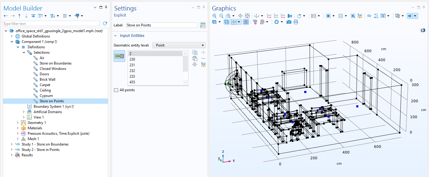 A black wireframe rendering of a room and its contents are shown with some points highlighted in blue.
Several points (receiver points) where the solution is stored are selected.
A black wireframe rendering of a room and its contents are shown with some points highlighted in blue.
Several points (receiver points) where the solution is stored are selected.
Physics Configurations
Hardware acceleration can be enabled from the Pressure Acoustics, Time Explicit interface by selecting the Use accelerated solver formulation option (shown below). This setting adds a Hardware Acceleration node to the solver that uses a GPU accelerated formulation when the Compute residual on GPU option is selected (default) and a CPU accelerated formulation otherwise. If the settings in the Pressure Acoustics, Time Explicit interface were changed, reset your study to the default so the settings for the Hardware Acceleration node are updated.
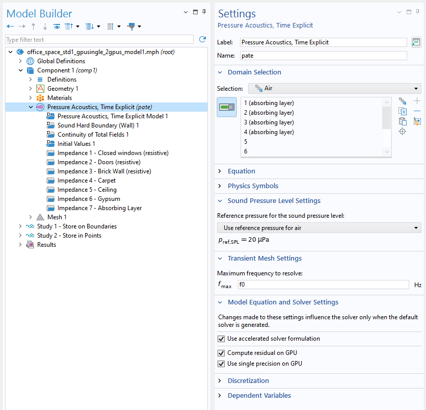 The user interface showing the settings window for the Pressure Acoustics, Time Explicit interface.
Enable the accelerated solver formulation to run on a GPU.
The user interface showing the settings window for the Pressure Acoustics, Time Explicit interface.
Enable the accelerated solver formulation to run on a GPU.
Mesh Configurations
When you create a Physics-controlled mesh, the Number of mesh elements per wavelength list is set to the Automatic option, which uses a conservative 1.5 elements per wavelength set in the Maximum frequency to resolve field (see image above). The Physics-controlled mesh option will also use the necessary mesh optimization settings.
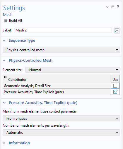 The settings window for a physics-controlled mesh.
A settings window for a physics-controlled Mesh node with the Number of mesh elements per wavelength list set to Automatic.
The settings window for a physics-controlled mesh.
A settings window for a physics-controlled Mesh node with the Number of mesh elements per wavelength list set to Automatic.
For large models, you may be able to reduce the computational cost by choosing the User-Defined option in the Number of mesh elements per wavelength list and entering 1.2–1.3 elements per wavelength.
If the User-controlled mesh option is used for the sequence type, then in the Element Quality Optimization section for a Free Tetrahedral mesh, select the Avoid elements that are too small option and set Optimization level to High. This setting alone can make a model solve much faster, as small mesh elements will be removed. In this case, use a Size node to set the Maximum element size parameter so that there are 1.5 to 1.2 elements per wavelength of the frequency with the shortest wavelength.
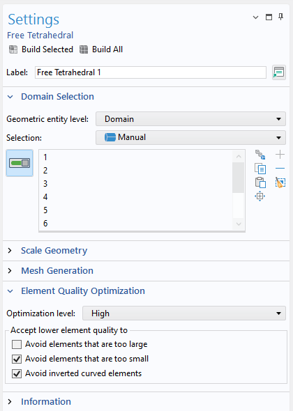 The Free Tetrahedral mesh Settings window with the Domain Selection and Element Quality Optimization sections expanded.
The Element Quality Optimization section in the Free Tetrahedral mesh Settings window offers options that can help you refine your mesh.
The Free Tetrahedral mesh Settings window with the Domain Selection and Element Quality Optimization sections expanded.
The Element Quality Optimization section in the Free Tetrahedral mesh Settings window offers options that can help you refine your mesh.
The size and therefore the number of your mesh elements have a significant impact on solution time. In time-explicit formulations, the solver sets the time step so that the wave will not skip over any elements in a single step, meaning the smallest elements force your entire model to use more time steps and thus take longer to solve. You can investigate the elements controlling the time steps with a Cell Wave Time Scale plot, which you can add from Results > Result Templates. The Cell Wave Time Scale plot shows a quantity proportional to the internal time step taken by the solver, which can help you identify which elements are driving the additional time steps.
Note: Rather than solving your entire model, you can use the Get Initial Values feature to gather sufficient information for Cell Wave Time Scale plots and investigate the elements.
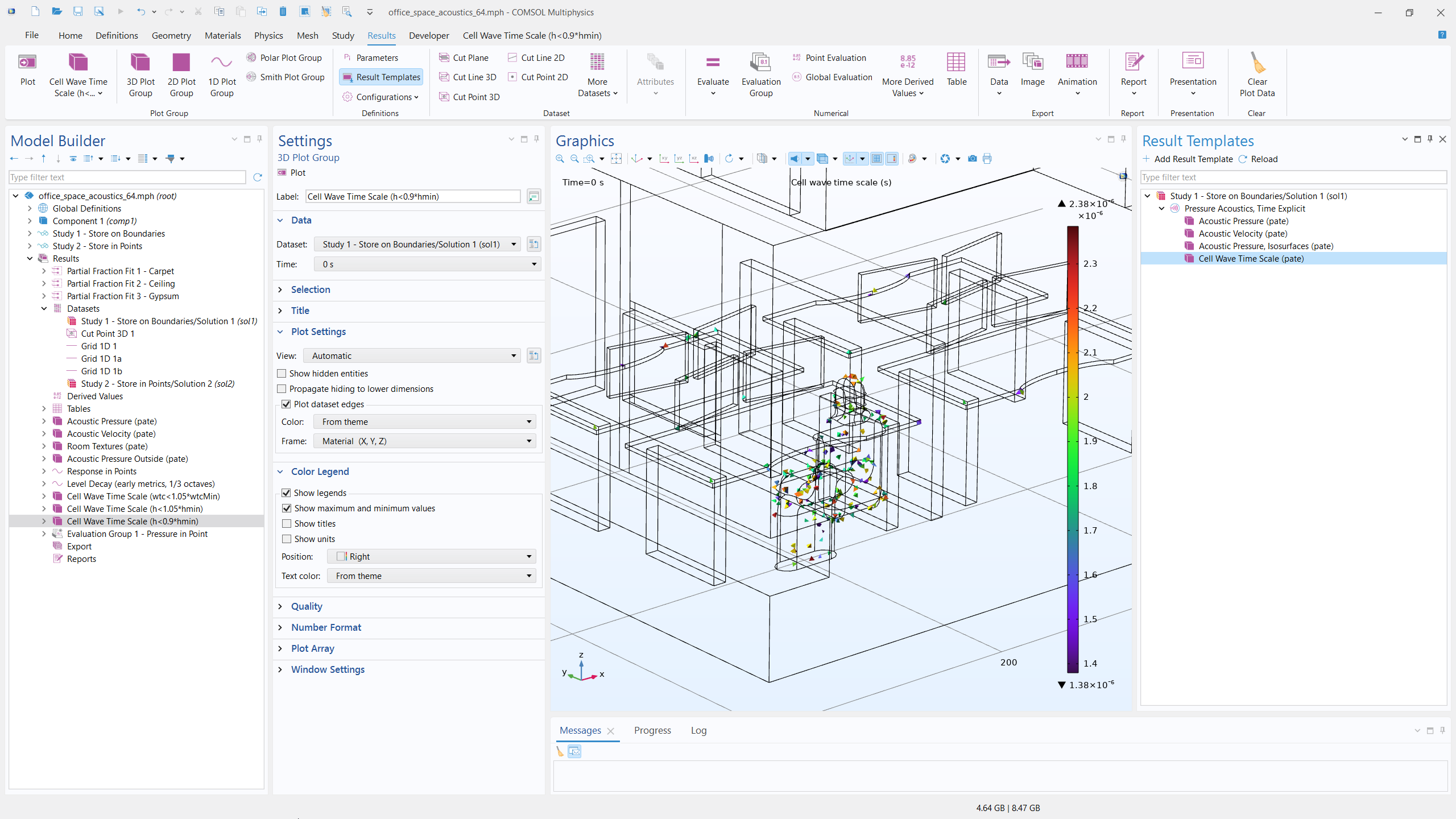 An office model in the Graphics window, with colored triangles plotted onto the wireframe of a person inside the office.
The Cell Wave Time Scale plot shows some of the small elements that are slowing down the computations.
An office model in the Graphics window, with colored triangles plotted onto the wireframe of a person inside the office.
The Cell Wave Time Scale plot shows some of the small elements that are slowing down the computations.
Study Configurations
When setting up the Time Dependent study step, it’s important to set the necessary temporal resolution (e.g., a given sampling frequency) in the Output times field for the Time Dependent solver. Note that output times are distinct from internal time steps.
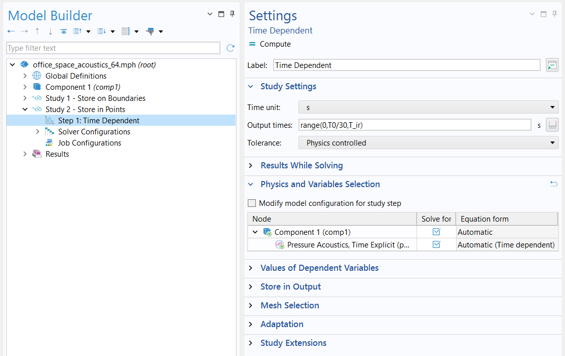 The output times are set in the Settings window for the Time Dependent study step.
The solution is stored using 30 points per period (of the maximum frequency), and the model is run to T_ir (0.4 s).
The output times are set in the Settings window for the Time Dependent study step.
The solution is stored using 30 points per period (of the maximum frequency), and the model is run to T_ir (0.4 s).
As we mentioned earlier, the selections created in the Definitions workflow step can be used in the Store in Output section of the Time Dependent solver. Choose your selections by opening the list for each interface in the Output column, picking Selection, and adding your desired selections of points or surfaces to the list. This step will help you avoid unnecessary data communication.
 A dropdown list in the Output column of a table is expanded, with the Selection option highlighted.
The Store in Output section saves the necessary data based on the desired selection.
A dropdown list in the Output column of a table is expanded, with the Selection option highlighted.
The Store in Output section saves the necessary data based on the desired selection.
Batch Commands to Run COMSOL Multiphysics® with Different GPU Configurations
As we stated earlier, COMSOL Multiphysics® version 6.4 update 1 introduced multi-GPU support for the Pressure Acoustics, Time Explicit interface. The COMSOL batch command enables you to run COMSOL Multiphysics® from the command line without opening the UI, such as in the following examples, which show how to use the batch command on a machine with four GPUs.
Assume the machine has four NVIDIA GPUs and 32 CPU cores.
Case 1: Single GPU
On Linux®, you can run a model using one GPU with:
comsol batch -inputfile example.mph -hwacc gpusingle
On Windows®, the equivalent command is:
comsolbatch -inputfile example.mph -hwacc gpusingle
These commands tell COMSOL® to solve example.mph without opening the UI and to use single‑precision GPU acceleration. COMSOL® will automatically choose which GPU to use.
Case 2: Multiple GPUs on the Same Machine
To use more than one GPU on a single machine, COMSOL® must be started in distributed mode using MPI, which requires a floating network license.
On Linux®:
comsol batch -nn 2 -nnhost 2 -np 16 -inputfile example.mph -hwacc gpusingle -clusterstorage shared
On Windows®:
mpiexec -n 2 comsolclusterbatch.exe -np 16 -inputfile example.mph -hwacc gpusingle -clusterstorage shared
This command starts 2 MPI processes on the same machine, each using 16 CPU cores. The example.mph model is solved using GPU single precision, and each MPI process writes its own output files to disk. On Linux®, Intel MPI is installed with COMSOL Multiphysics®. On Windows®, Microsoft MPI must be installed separately.
See the COMSOL Commands for more information, or contact support for assistance with your specific configuration.
The Office Space Model
The Acoustics of an Open-Plan Office Space model is set up to solve two studies. A source pulse with center frequency 500 Hz is used. The model resolves frequencies up to f0 = 750 Hz, defining the period T0 = 1/f0. The first study solves for 20 periods (20*T0) and stores the solution twice per period on all boundaries. These results are used for visualization of the early sound propagation. The second study solves the model for 0.4 s and stores the solution 30 times per period in the 8 microphone locations.
The model is solved on one and two NVIDIA RTX 6000 Ada GPUs, respectively. The solution time, using best practices, is as follows:
| 1x NVIDIA RTX 6000 Ada | 2x NVIDIA RTX 6000 Ada | |
|---|---|---|
| Study 1 | 15 min 28 s | 8 min 32 s |
| Study 2 | 3 h 40 min | 2 h 3 min |
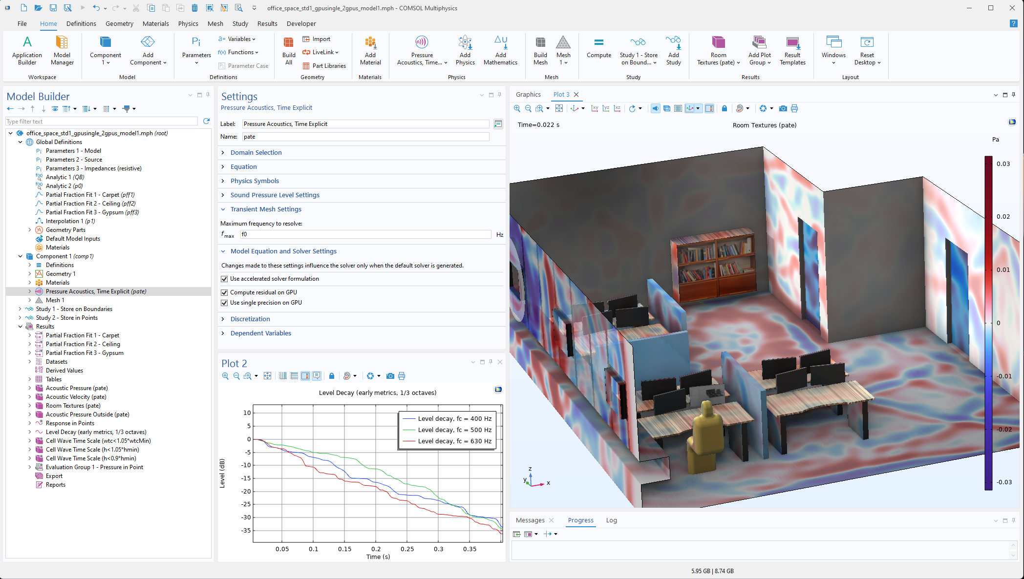 An office model is shown in the Graphics window, with red and blue plotted on the surfaces.
Settings for the Acoustics of an Open-Plan Office Space tutorial model.
An office model is shown in the Graphics window, with red and blue plotted on the surfaces.
Settings for the Acoustics of an Open-Plan Office Space tutorial model.
Further Learning
See the "Modeling Pressure Acoustics" course to learn more about modeling pressure acoustics. Additionally, check out the following models:
- Acoustics of an Open-Plan Office Space
- Car Cabin Acoustics — Transient Analysis
- Wave-Based Time-Domain Room Acoustics with Frequency-Dependent Impedance
- Chamber Music Hall — Wave Based
Linux, Linux Standard Base, and LSB are trademarks or registered trademarks of Linus Torvalds in the U.S. and other countries. Microsoft, Windows, and Windows Server are either registered trademarks or trademarks of Microsoft Corporation in the United States and/or other countries. NVIDIA is a trademark and/or registered trademark of NVIDIA Corporation in the U.S. and/or other countries.
Submit feedback about this page or contact support here.