Studies and Solvers Updates
COMSOL Multiphysics® version 6.0 includes improved mesh adaptation for curl element formulations, performance improvements for cluster computations, and Component Mode Synthesis for modal reduction. Learn about all of the updates relating to studies and solvers below.
Improved Mesh Adaptation for Curl-Element Formulations
The mesh adaptation method has been extended with a new interpolation error estimator. This makes more efficient mesh adaptation possible for the curl-element formulations used in the RF Module. Both curl elements of type 1 and 2 are supported. A new Frequency Domain, RF Adaptive Mesh study makes the workflow much easier when setting up mesh adaptation for modeling microwave and millimeter-wave antennas and circuits.

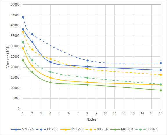
Performance Improvements for Cluster Computing
The core machinery for finite element assembly has been improved for cluster computing. Data locality and mesh element partitioning has been improved, both contributing to an overall improved performance for cluster computing. These improvements apply to both multigrid and domain decomposition preconditioners.

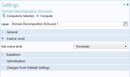
New Coarse Grid Method for Domain Decomposition
It is now possible to create a coarse grid correction with the Nicolaides method. This method can be used to construct a very aggressive coarsening down to just a few unknowns. The method can be used to strike the balance between robustness and performance for the domain decomposition solver, where a standard coarsening method can be too expensive of an alternative and where running without a coarse grid does not work.
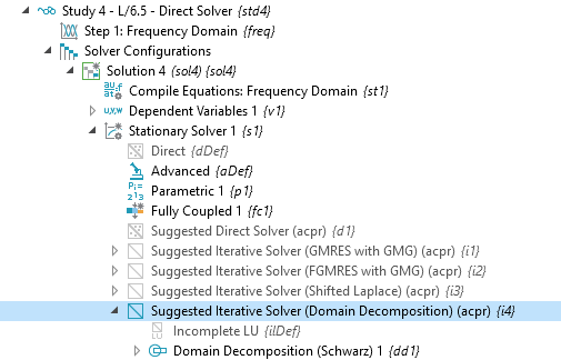
New Domain Decomposition Method for Pressure Acoustics
It is now possible to solve large-scale pressure acoustics (Helmholtz problems) with the Domain Decomposition (Schwarz) method. This method is using the Shifted Laplace method together with the same absorbing boundary conditions for the internal overlapping boundaries as is used for the nonoverlapping Schur method. The advantage with this method is that multigrid can be used as a domain solver and a coarse grid is not needed for the domain decomposition method.
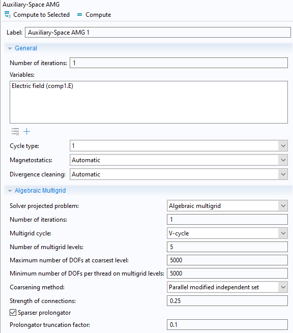
New Algebraic Multigrid Methods
The standard, or classical algebraic, multigrid method has been extended with a new coarsening method called Parallel modified independent set. This method supports cluster computing. Furthermore, the Auxiliary-Space AMG method has been extended to support complex-valued curl-element formulations.
Improvements to Batch and Cluster Computing
The Batch and Cluster Computing study types, including the sweep variants Batch Sweep and Cluster Sweep, have been improved. For Batch and Cluster Computing, you can now synchronize the solutions and accumulated probe tables from the batch process. A new cleanup method is available that removes synchronization data for the external process or processes. These new methods are enabled, by default, for the study types Batch and Batch Sweep.
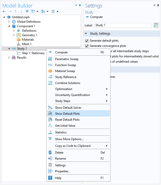
New Ways to Generate Default Plots
You can now generate, or reset, the default plots before solving. Right-click on any study and choose either Show Default Plots or Reset Default Plots.
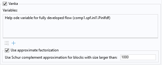
New Approximate Schur Complement Method for the Vanka Solver
The Vanka solver is extended with a new approximate factorization method for its matrix blocks. When using the Block solver method Direct, stored factorization, there is now an option to Use approximate factorization that is using a Schur complement approximation for larger blocks. This method can save significant memory and CPU time for large blocks, as encountered in, for example, large 3D fluid flow models with the fully developed inflow boundary conditions. This method is available both from the Vanka solver as well as from the SCGS solver with the Vanka option enabled.
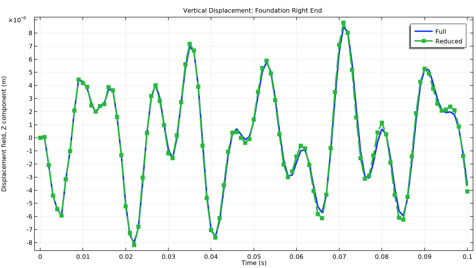
Craig–Bampton Method for Model Reduction
Component mode synthesis, based on the Craig–Bampton method, is now available in the Structural Mechanics Module, Multibody Dynamics Module, and Rotordynamics Module. The Craig–Bampton method is used to extend the Modal method for Model Reduction, which can now have model inputs in the constraints. The method takes so-called constraint modes as input, as an extension of the standard modal basis. These modes can be computed in a separate standard Stationary or Parametric Sweep study. Furthermore, modal-reduced-order models now support both a stateless and a stateful form. The stateful form exposes the reduced system of equations to the COMSOL equation machinery, which makes coupling of reduced models to other equations easier. As a side effect of this, the modal degrees of freedom become available for postprocessing or further modeling.

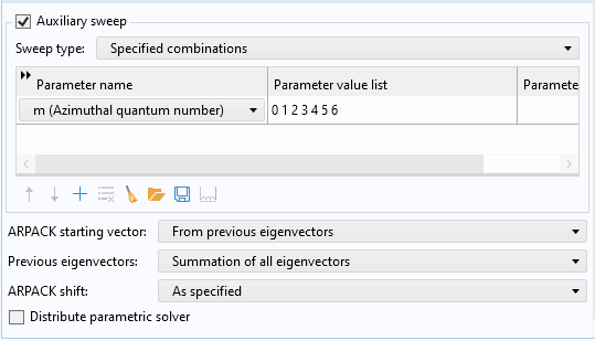
Reuse of Solution for Parametric Eigenvalue Problems
It is now possible to select the start vectors when solving parametric eigenvalue problems. This functionality can save computational time for eigenvalue problems with solutions that are smoothly varying with a change in the parameter. Examples can be found in the Semiconductor Module, in models that use the Schrödinger-Poisson interface. With the Eigenvalue search method set to Manual, you can often reduce the number of iterations by at least 50%.
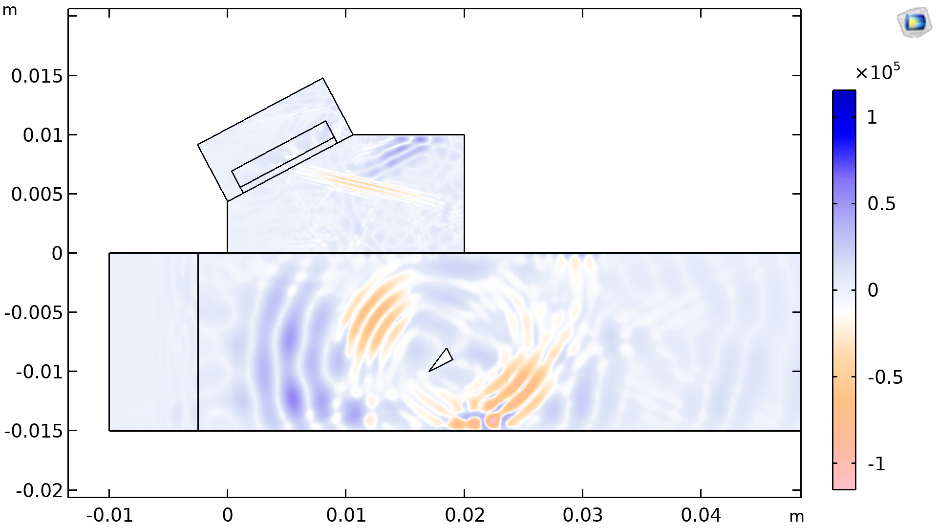
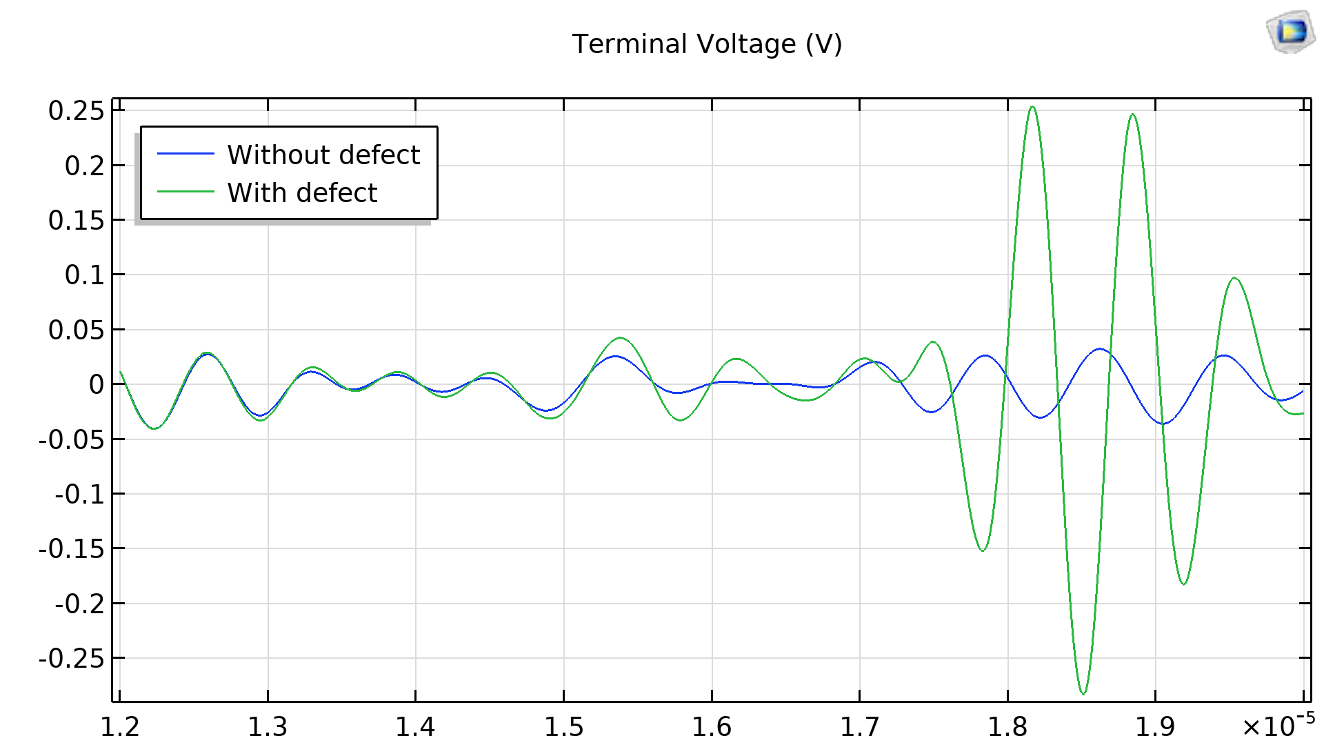
Time-Explicit Multiphysics dG-FEM Hybrid Method
It is now possible to solve for elastic waves coupled to a piezoelectric domain using a time-explicit discontinuous Galerkin-FEM hybrid method. The piezoelectric part of the problem is formulated with the finite element method and is coupled to elastic waves formulated with the time-explicit nodal discontinuous method. The method can handle large elastic domains and is applicable to the design of ultrasound-based medical devices.