Subsurface Flow Module Updates
For users of the Subsurface Flow Module, COMSOL Multiphysics® version 6.0 brings improved handling of porous materials, nonisothermal flow in porous media, and source terms for the Shallow Water Equations interface. Learn more about these updates below.
Nonisothermal Flow in Porous Media
The new Nonisothermal Flow, Brinkman Equations multiphysics interface automatically adds the coupling between heat transfer and fluid flow in porous media. It combines the Heat Transfer in Porous Media and Brinkman Equations interfaces. You can see this new feature in the existing Free Convection in a Porous Medium tutorial model.
Heat Transfer in Porous Media Improvements
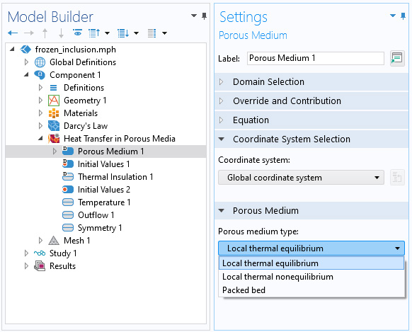
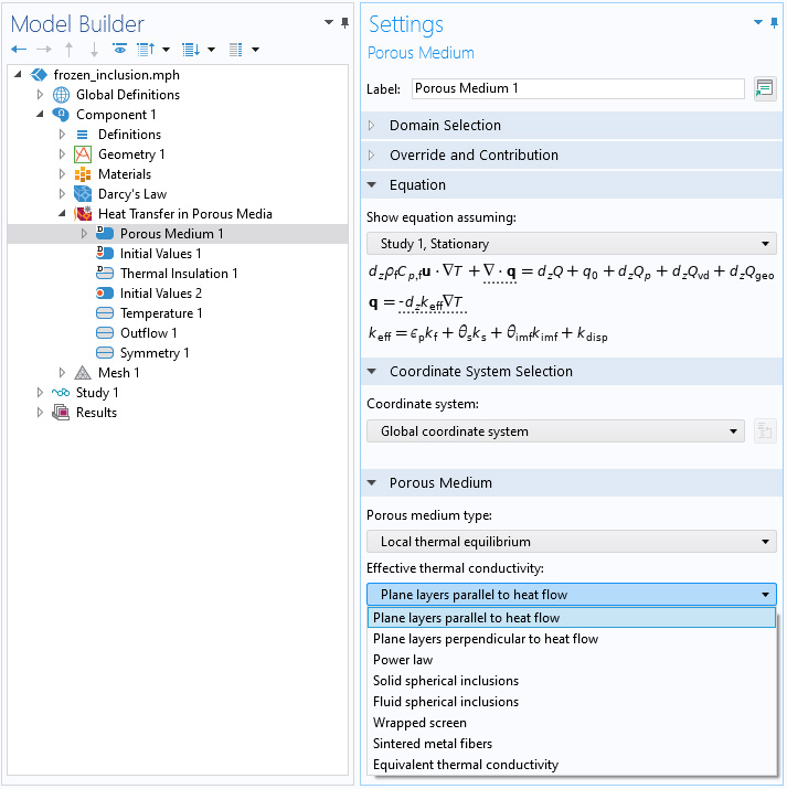
The heat transfer in porous media functionality has been revamped to make it more user friendly. A new Porous Media physics area is now available under the Heat Transfer branch and includes the Heat Transfer in Porous Media, Local Thermal Nonequilibrium, and Heat Transfer in Packed Bed interfaces. All of these interfaces are similar in function, the difference being that the default Porous Medium node within all these interfaces has one of three options selected: Local thermal equilibrium, Local thermal nonequilibrium, or Packed bed. The latter option has been described above and the Local Thermal Nonequilibrium interface has replaced the multiphysics coupling and corresponds to a two-temperature model, one for the fluid phase and one for the solid phase. Typical applications can involve rapid heating or cooling of a porous medium due to strong convection in the liquid phase and high conduction in the solid phase like in metal foams. When the Local Thermal Equilibrium interface is selected, new averaging options are available to define the effective thermal conductivity depending on the porous medium configuration.
In addition, postprocessing variables are available in a unified way for homogenized quantities for the three types of porous media. View the new porous media additions in these existing tutorial models:
Greatly Improved Handling of Porous Materials
Porous materials are now defined in the Phase-Specific Properties table in the Porous Material node. In addition, subnodes may be added for the solid and fluid features where several subnodes may be defined for each phase. This allows for the use of one and the same porous material for fluid flow, chemical species transport, and heat transfer without having to duplicate material properties and settings.

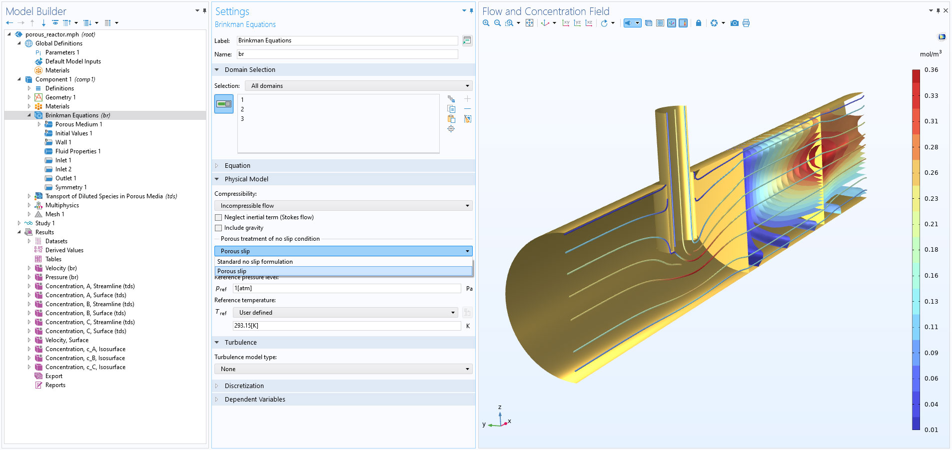
Porous Slip for the Brinkman Equations
The boundary layer in flow in porous media may be very thin and impractical to resolve in a Brinkman equations model. The new Porous slip wall treatment option allows you to account for walls without resolving the full flow profile in the boundary layer. Instead, a stress condition is applied at the surfaces, yielding a decent accuracy in the bulk flow by utilizing an asymptotic solution of the boundary layer velocity profile. The functionality is activated in the Brinkman Equations interface Settings window and is then used for the default wall condition. This new feature may be used in most models involving subsurface flow described by the Brinkman equations and where the model domain is large.
Source Terms for the Shallow Water Equations Interface
The shallow water equations give a 1D or 2D approximation of shallow flows by averaging along the depth. Rain, local upwellings, pumping devices, or boundary stresses have to be introduced as source terms in the model equations. This was previously possible through the equation view, but the ability to add momentum and mass sources is now available as predefined settings in the flow interface.
New Tutorial Model
COMSOL Multiphysics® version 6.0 brings one new tutorial model to the Subsurface Flow Module.
Glacier Flow: A 2D Study of Cold and Temperate Glaciers
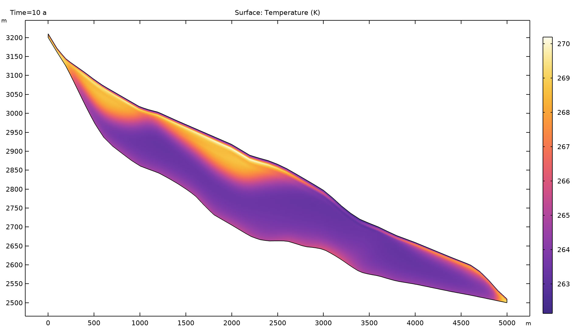
Application Library Title:
glacier_flow_2d
Download from Application Gallery