COMSOL Multiphysics^® 6.1 Release Highlights

Multibody Dynamics Module Updates

For users of the Multibody Dynamics Module, COMSOL Multiphysics^® version 6.1 introduces contact modeling improvements, an interface for analyzing wires and cables, and a new method for enforcing continuity between boundaries in assemblies. Read about these updates and more below.

Contact Modeling Enhancements

Several additions and improvements have been made to the contact modeling functionality, affecting both performance and capabilities.

• A new, faster contact search algorithm has been implemented. It is particularly advantageous for large 3D models.
• Nitsche's method, a new method for formulating contact equations, has been added. It is a robust method that does not add any extra degrees of freedom.
• New, more stable formulations of the contact equations have been added for all contact models.
• Support for self-contact has been improved. The formulation is now symmetric between the two sides of the contact pair.

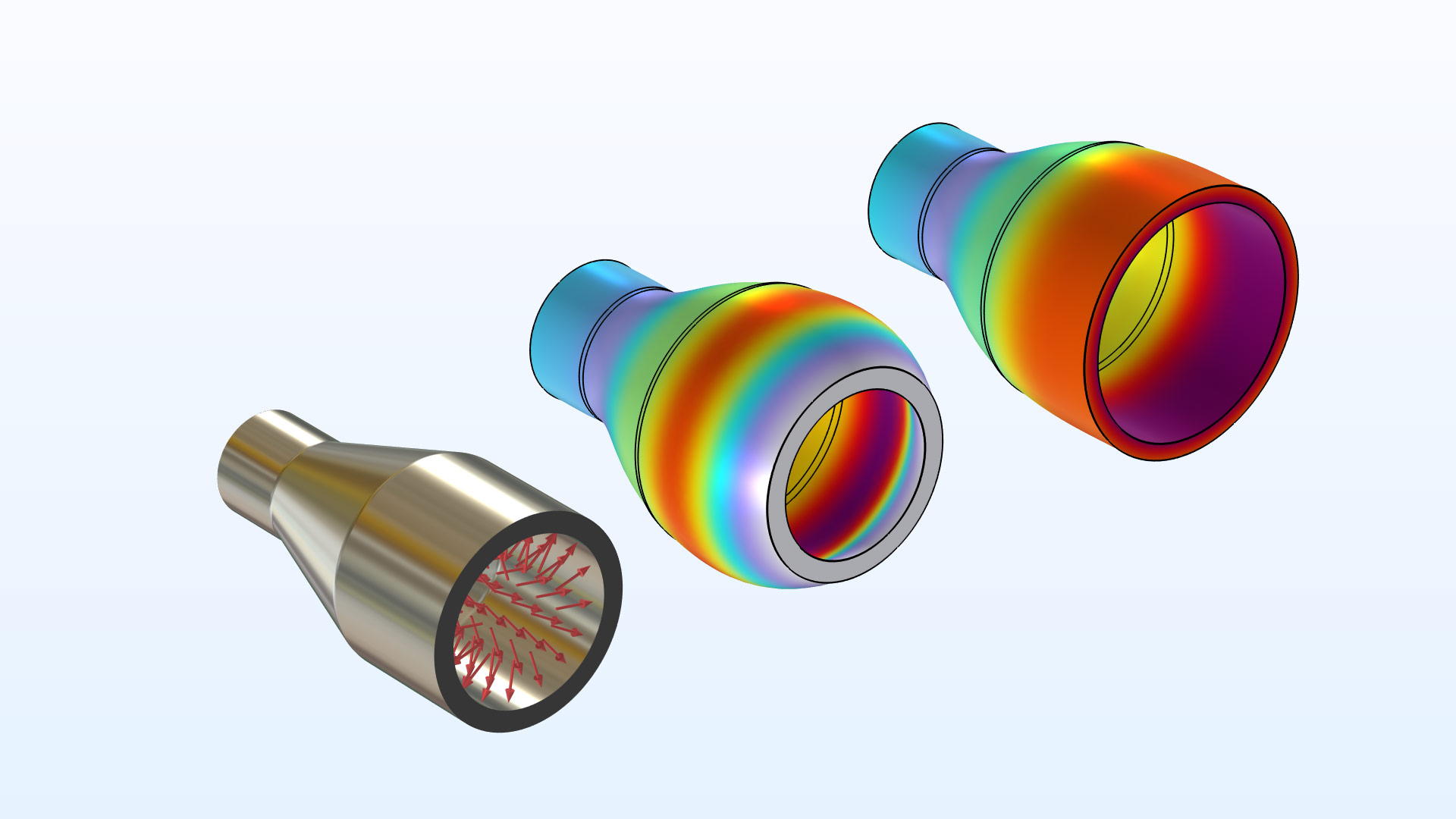
Animation of an elastoplastic pipe forced into a conical hole. Self-contact occurs in several places.

Physics Interface for Wires

A new physics interface, Wire, has been added. It is intended for the analysis of cables or wire systems, separately or in conjunction with other types of structures. The wires can be prestressed or sagging under self-weight. You can see this new functionality in the following models:

• truss_tower_buckling_guys (new)
• vibrating_string
• hanging_cable

Forces in a grid of wires under gravity load when the support points are moved inward. Part of the grid comes to rest on a rigid surface.

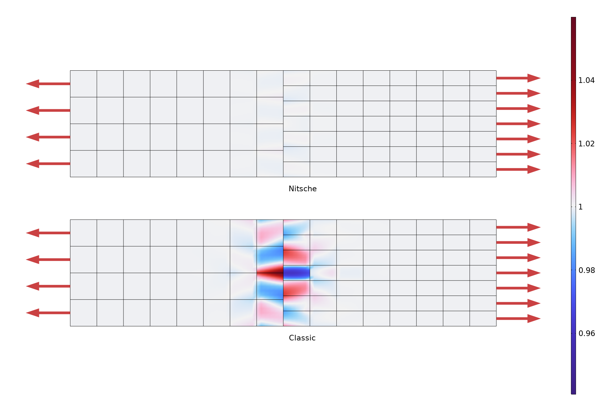
New Method for Connecting Assemblies

A new method for enforcing continuity between boundaries in assemblies has been added: Nitsche's method. The new method has two important advantages when compared with classical pointwise constraints:

1. It causes significantly less local disturbances in the solution when the meshes on the two sides
   are not conforming.
2. Since no constraints are added, the numerically sensitive and sometimes computationally heavy
   constraint-elimination step is avoided.

Comparison of local stress disturbance when using either a classical constraint or the new Nitsche's method for connecting mismatching meshes.

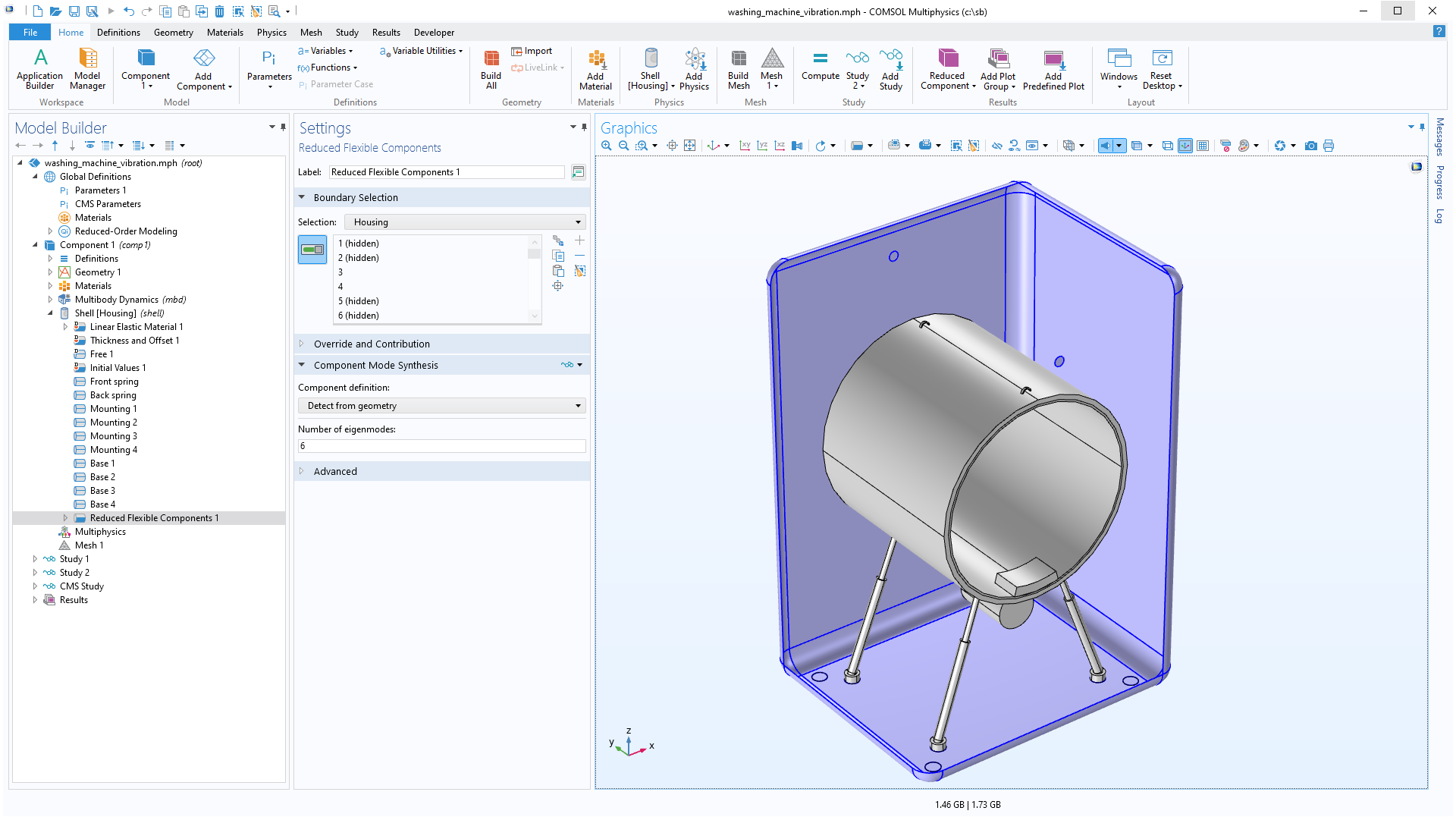
Component Mode Synthesis Enhancements

With the Structural Mechanics Module, it is now possible to use shell elements in component mode synthesis (CMS) analyses. There are also several general improvements that makes it easier to set up models for CMS analyses.

In this example — a study of the dynamics of a washing machine — the analysis time is reduced by a factor of 2 when the shell representing the enclosure is reduced to a CMS component.

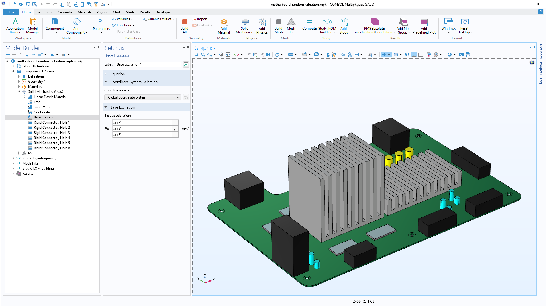
Base Excitation

It is common that the dynamic loading on a structure consists of a certain acceleration of all its support points. An example of this is when a part is attached to a shaker table for testing. This type of loading can now be more naturally described using the new Base Excitation feature.

An example of base excitation, where a structure has a uniform prescribed acceleration at all bolt holes. Base excitation is a property of the entire model, so this feature does not have any selections.

Loads Given as Resultant

For boundary loads and sets of point loads, you can now specify the total force and moment with respect to a given point by selecting the Resultant option from the Load type list. This makes it easier to apply load resultants without either imposing artificial constraints or making long calculations of the actual load distributions. It is possible to control the assumed shape of the load distribution.

A bending load given as a moment resultant is applied to the end of a beam, modeled as a 3D solid. The actual load distribution is shown by arrows.

Improvements for Rigid Connectors

The Rigid Connector is an important tool for abstract modeling, such as when applying loads and connecting objects. Its functionality has been augmented in three respects:

1. It is now possible to disconnect selected degrees of freedom, such as in directions given by a local coordinate system. With this option, it is possible to release excessive constraints and reduce local stress concentrations.
2. For two-point rigid connectors in 3D, it is possible to automatically suppress the potential rotational singularity.
3. As a new default, the degrees of freedom that are generated by rigid connectors are now grouped together in the study sequence. This can dramatically reduce the number of nodes in the model tree and makes it easier to apply manual scaling for convergence tolerance. The same change also applies to the Attachment feature.

The effects of released degrees of freedom. The reducer with internal pressure has a rigid connector at the end, as shown in the brown surface in the leftmost figure. As shown in the middle figure, with a standard formulation, the assumption about rigidity will keep the radius constant. In the rightmost figure, the radial displacement is released in the rigid connector. It is still possible to apply loads in any direction or connect to other domains.

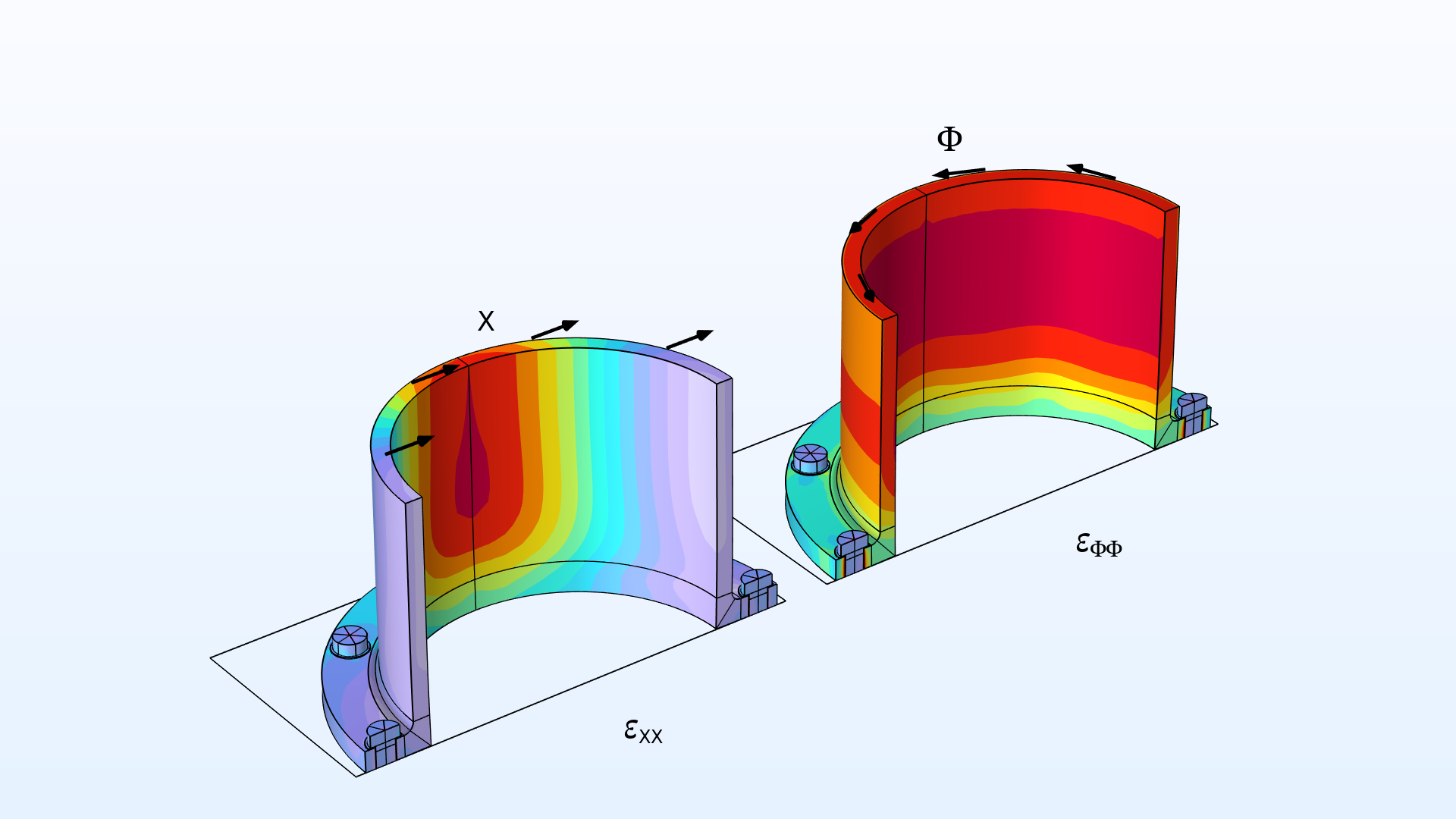
Results in Local Coordinate Systems

It is now easy to define an arbitrary number of local coordinate systems by adding Local System Results nodes for the evaluation of common result quantities. Among the available transformed quantities, you will find stresses, strains, displacements, and material properties.

Direct strain in the global x-direction and the azimuthal direction for a geometry with cylindrical symmetry.

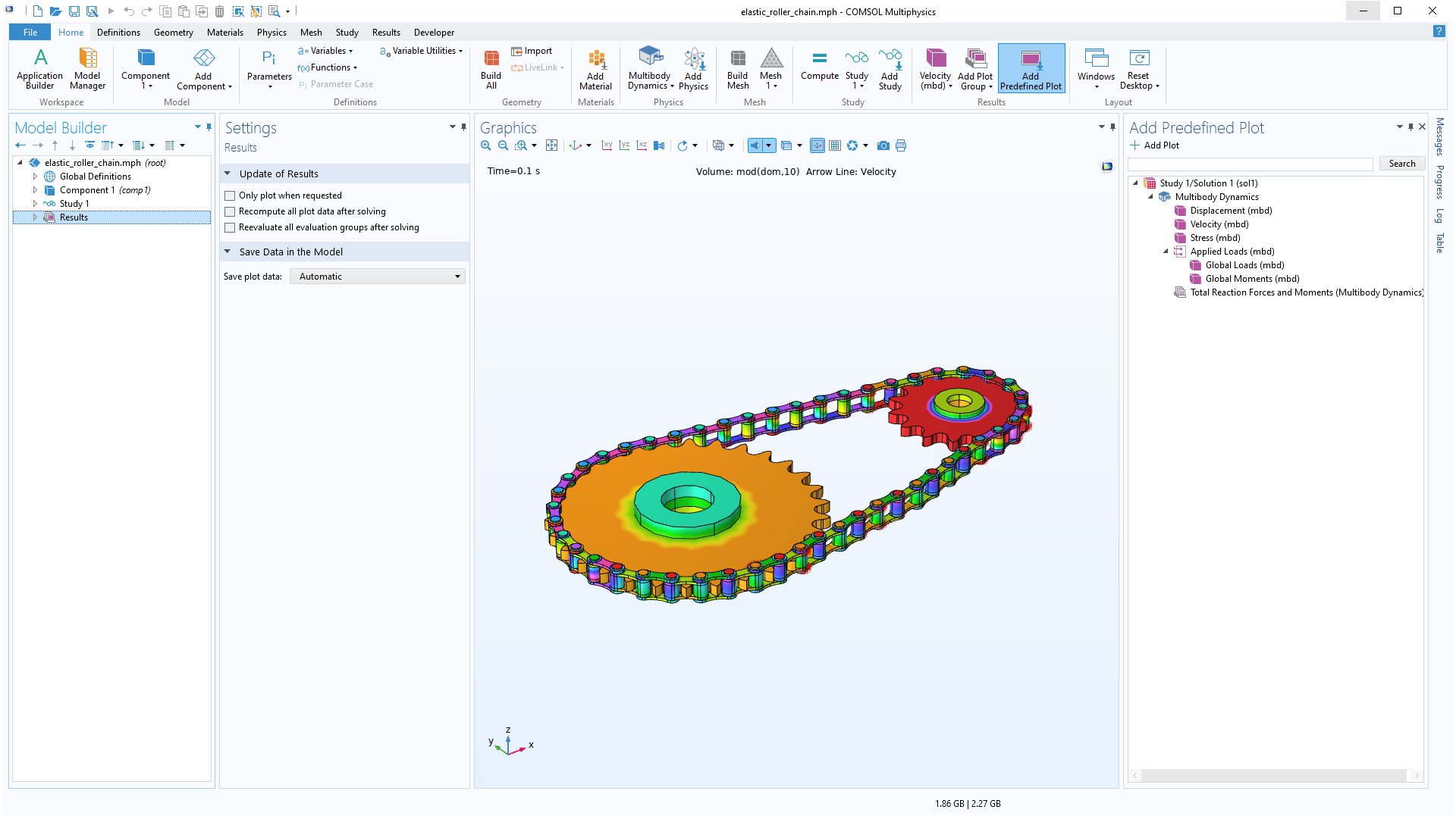
Predefined Plots

A new general functionality for predefined plots has been added. A predefined plot is similar to a default plot, but with the important difference that it is not added to the Model Builder until the user selects to do so. This has three advantages:

1. The number of default plots that are generated for each study has been decreased significantly.
2. Several new useful plots are available from the Add Predefined Plot menu, in addition to the default plots in previous versions.
3. Result plots for intermediate study steps — for example, the loading step in a prestressed dynamic analysis — are directly available.

The Add Predefined Plot window for one of the models in the Application Libraries.