Modeling with PDEs: Lower Dimensions and ODEs and DAEs Interfaces
Here in Part 5 of this 11-part course on modeling with partial differential equations (PDEs) in COMSOL Multiphysics®, you will learn how to use the interfaces for specifying PDEs on boundaries and edges. You will also see some very important degenerate cases of PDEs where many of the coefficients are zero, and you will learn how this can be used to model distributed ordinary differential equations (ODEs), differential-algebraic equations (DAEs), and algebraic equations.
Table of Contents
- The PDE Interfaces for Modeling in Lower Dimensions
- The Coefficient Form Boundary PDE
- Electric Currents in a Steel Tank
- Coupling PDEs of Different Dimensions
- Modeling Distributed ODEs and DAEs
- Modeling Distributed Algebraic Equations
- Field Continuity for Distributed ODEs and DAEs
- Further Learning
The PDE Interfaces for Modeling in Lower Dimensions
Many physical processes take place in thin structures, such as metallic shells or conductive membranes. It can be challenging to model these thin structures with a direct approach, where the structure, including its thickness, is represented by a CAD model and finite element mesh. This is because large aspect ratios can cause numerical problems with meshing and geometry analysis. Instead, thin structures can oftentimes be modeled as shells, without modeling the geometrical thickness of the structure. In such cases, the thickness can be treated as a physical property and represented as a kind of material property in the equations, which are implemented on the boundary of the structure. Through our example model, you will see how to use the Coefficient Form Boundary PDE interface to solve a partial differential equation in curved 3D shells.
As seen in other parts of this course, there are several easy-to-use predefined physics interfaces built into the software for various types of shell modeling. For example, in the AC/DC Module there are predefined Electric Currents in Shells and Electric Currents in Layered Shells interfaces, as shown in the figure below.
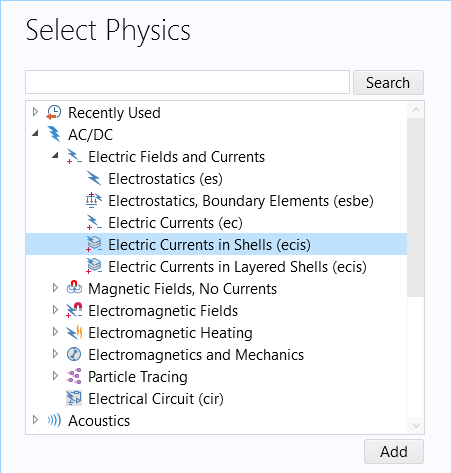
The Electric Currents in Shells physics interface in the AC/DC Module.
For educational purposes, we will show how to implement the Electric Currents in Shells interface using the Coefficient Form Boundary PDE interface. In the Select Physics page in the Model Wizard, the Lower Dimensions interfaces are available in the corresponding branch under the Mathematics branch, as shown in the figure below.
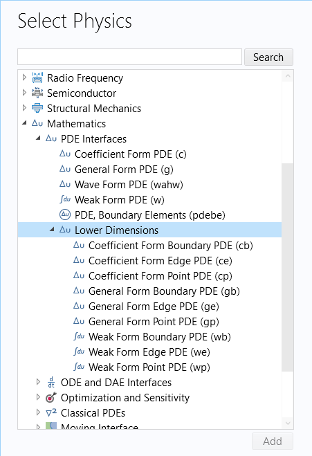
The interfaces for modeling PDEs in lower dimensions.
Note that not only can you define lower-dimensional equations on boundaries, but you can also define them along edges and at points. When considering PDE interfaces for lower-dimension equations, do not confuse the Coefficient Form Boundary PDE interface with the PDE, Boundary Elements interface. The Coefficient Form Boundary PDE is an interface for lower dimensions (boundaries) and is based on the finite element method, whereas the PDE, Boundary Elements interface is based on the boundary element method and is not available for lower-dimensional equations.
The Coefficient Form Boundary PDE
The Coefficient Form Boundary PDE is very similar in appearance to the Coefficient Form PDE defined for domains:

with the Neumann boundary condition:

and the Dirichlet condition:

In 2D, the vector  is a tangent vector to the boundary curve at its end points. In 3D, the vector is perpendicular to both the surface normal and the edge tangent vector.
The difference is that in the Coefficient Form Boundary PDE interface, the divergence and gradient are defined in terms of the tangential derivatives on the boundary. In addition, the boundary conditions are now defined (in 3D) on curves, or edges, rather than on surfaces. In 2D, the boundaries are points.
To get an intuitive understanding of the tangential versions of the divergence and gradient operators, consider an arbitrary vector,  , on a boundary surface in 3D, as shown in the figure below.
A generic vector on a surface in 3D.
We can get the projection  of this vector in the tangent direction of the surface by subtracting the component normal to the surface
  .
.
The normal component of is its projection on the surface unit normal  :
:

The tangential component of is:

By using matrix-vector notation we can also write this as:

where subscript  is the tangential component, superscript is the matrix transpose, and
  is the identity matrix.
The figure below shows an example with the three vectors: , , and .
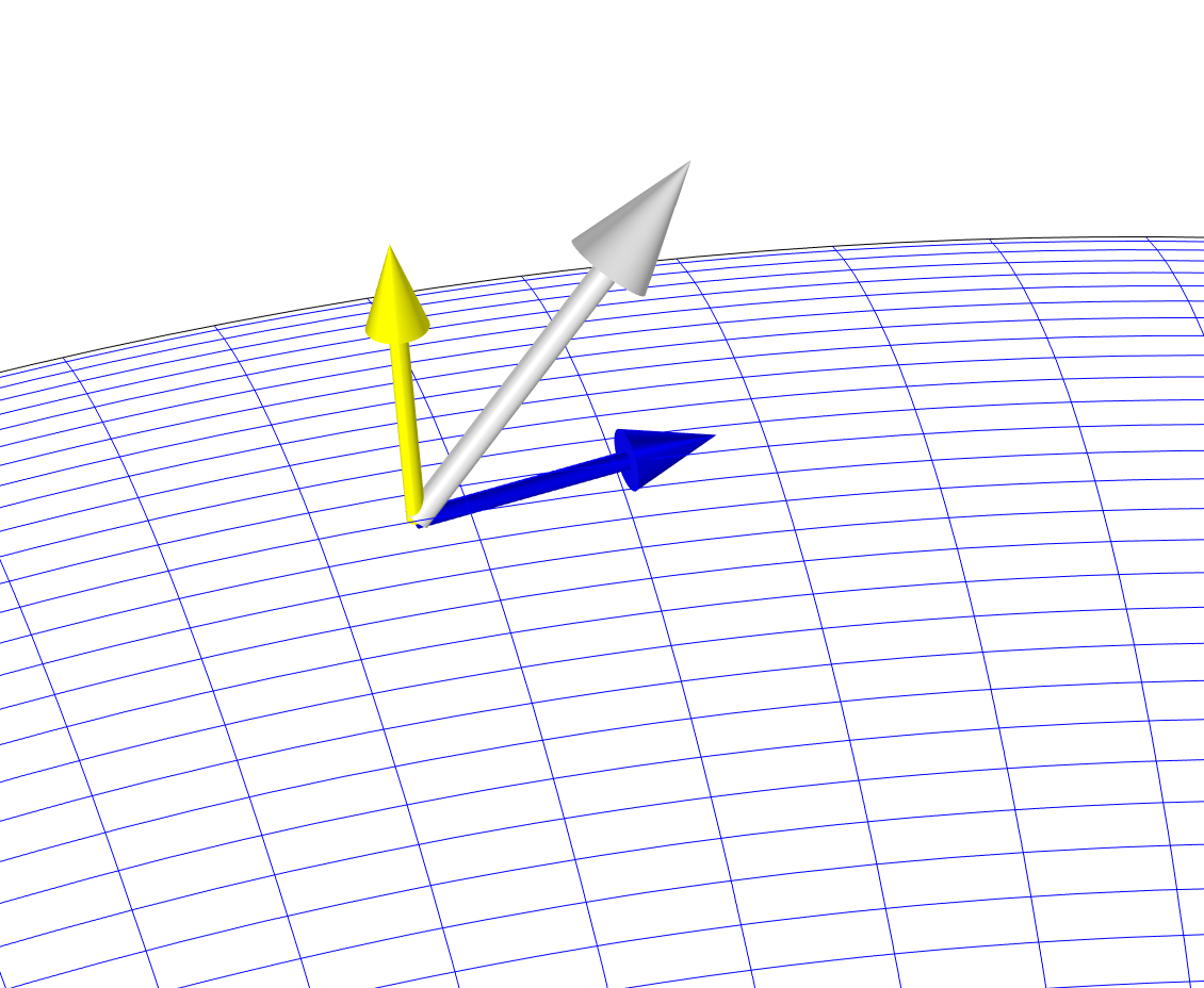 A surface with three 3D vectors that appear as yellow, gray, and blue arrows pointing outward in different directions.
The vectors (gray), (yellow), and (blue).
In the same way, we can get the tangential component of the gradient of a variable  as:
as:

and, similarly, the divergence of a vector  as:
as:

Here, we have assumed that the field is defined inside the surface as well as on both sides outside of the surface, so we can compute the derivatives without running into any problem. In the case where the field is only defined inside the surface, the generalized formula is still applicable.
This is the form of the gradient and divergence operators that is used in the Coefficient Form Boundary PDE interface. By formulating the PDE in terms of tangential derivatives, we can, for example, describe the convection–diffusion-reaction processes taking place in the tangential direction of a surface. Current conduction in a thin metallic shell is an example of such a process. Another important example is surface chemistry with adsorption and surface diffusion.
Electric Currents in a Steel Tank
In this example, we will analyze the electric currents in a steel tank. The steel tank, shown in the figure below, has two pipe connections. One is grounded and the other connects to a current source, modeled using a fixed voltage condition of 400 V. This model calculates the current density in the tank shell as well as the potential distribution across the surface.
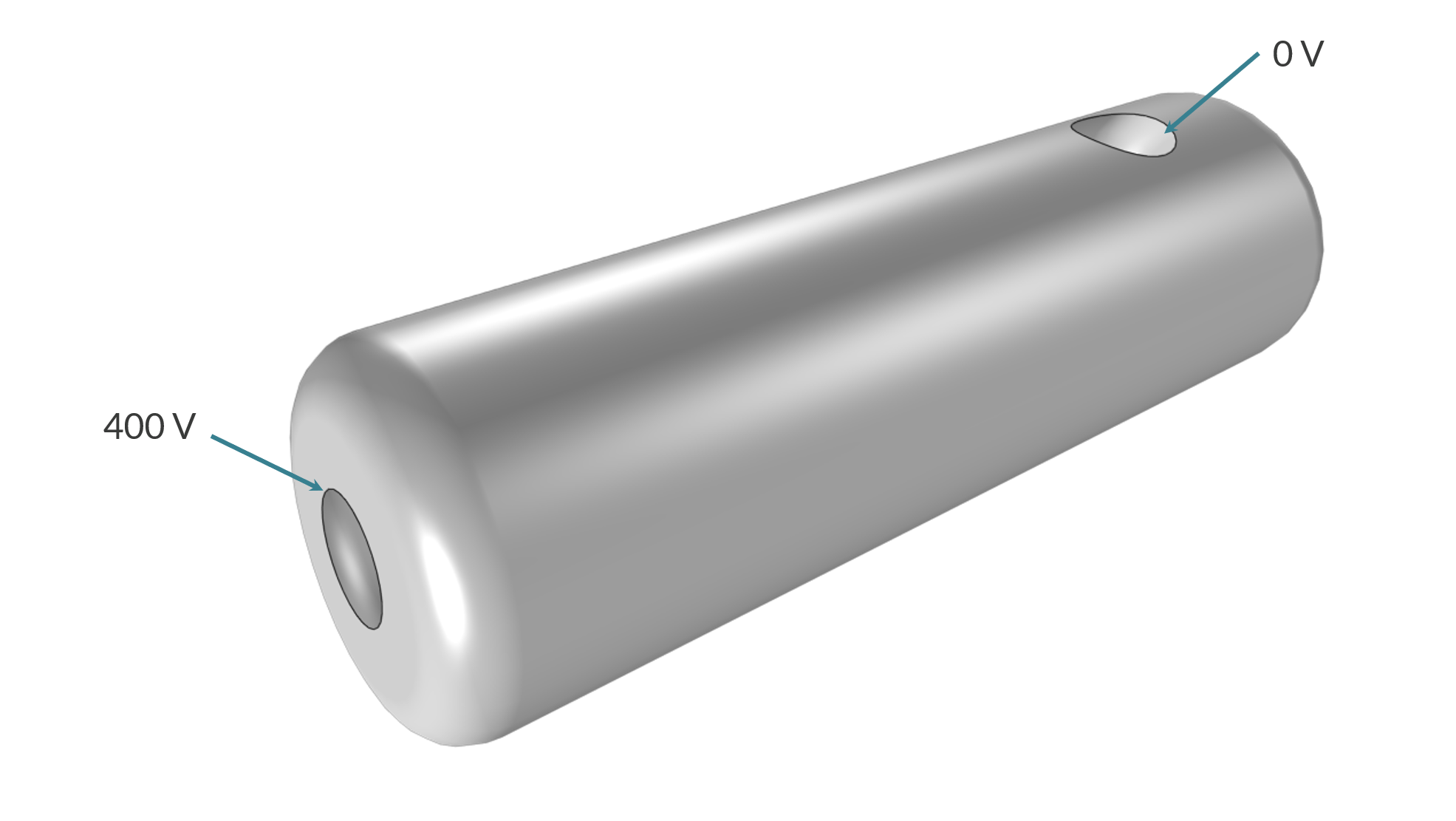 A steel tank model with 400 V and 0 V labeled.
The steel tank model configuration.
A steel tank model with 400 V and 0 V labeled.
The steel tank model configuration.
The equation for the stationary electric currents in a shell is:

where  is the electric potential,
  is the electric conductivity of the steel, and
  is the steel thickness. This extra factor for the steel thickness is how the geometrical thickness is encoded in the PDE, rather than as an explicit thickness that is physically represented in the CAD model. In this case, the CAD model does not have thickness; it is just a surface.
In this model, the parameters for conductivity and thickness are defined as global parameters, as shown in the figure below.
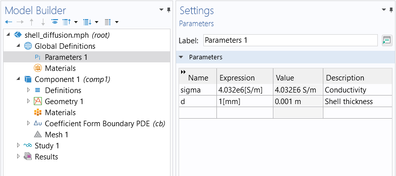
The global parameters for conductivity and shell thickness.
If we compare the equation
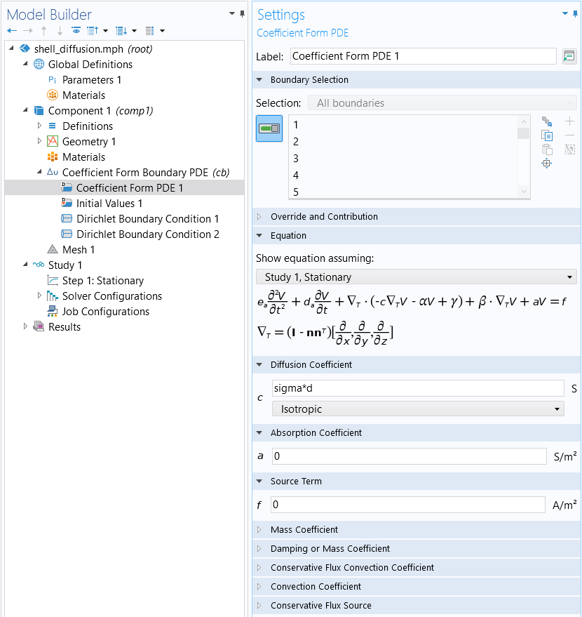
with the stationary version of the Coefficient Form Boundary PDE equation:

we see that:

and all other coefficients are zero. The figure below show these settings in the Coefficient Form Boundary PDE interface:
The boundary conditions are defined on the two sets of connected edges, as shown in the figures below.
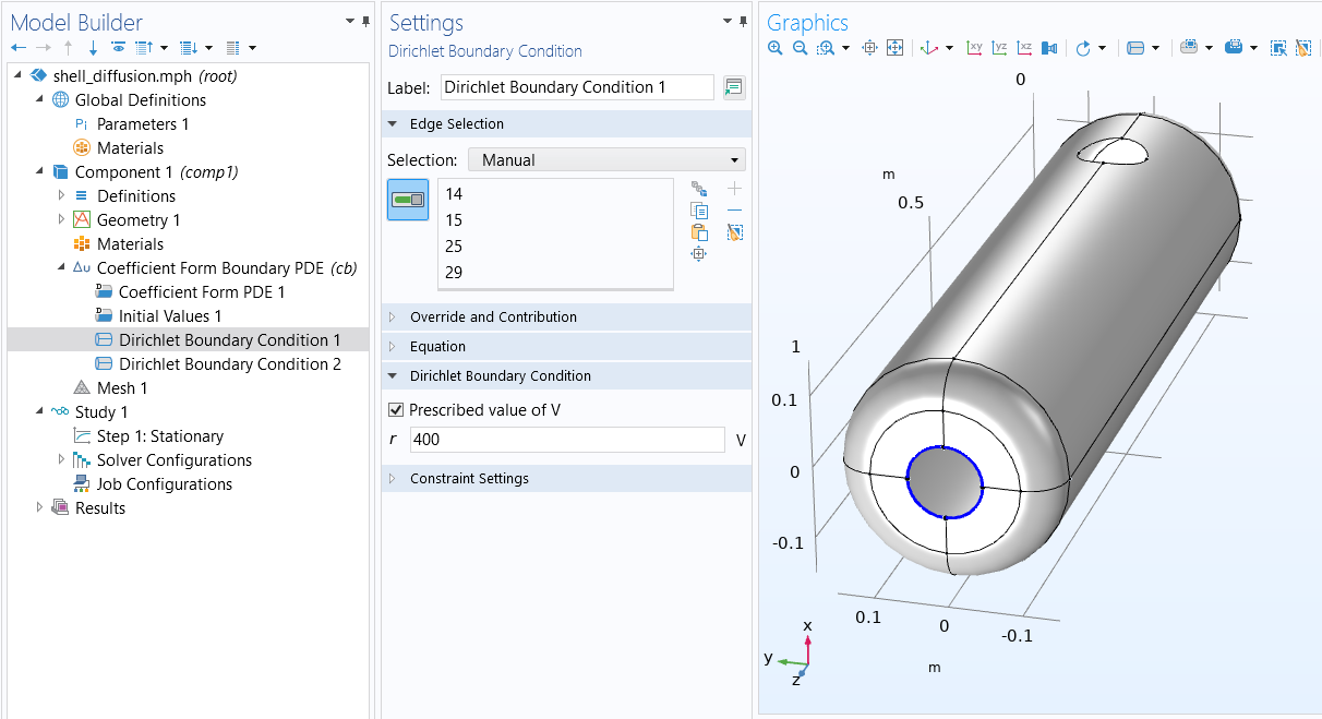 The Model Builder with Dirichlet Boundary Condition 1 selected, the corresponding Settings window with 400 V set, and the steel tank model in the Graphics window.
The Dirichlet condition for one of the boundaries where
The Model Builder with Dirichlet Boundary Condition 1 selected, the corresponding Settings window with 400 V set, and the steel tank model in the Graphics window.
The Dirichlet condition for one of the boundaries where  .
.
 The Model Builder with Dirichlet Boundary Condition 2 selected, the corresponding Settings window with 0 V set, and the steel tank model in the Graphics window.
The Dirichlet Boundary Condition for the other boundary where
The Model Builder with Dirichlet Boundary Condition 2 selected, the corresponding Settings window with 0 V set, and the steel tank model in the Graphics window.
The Dirichlet Boundary Condition for the other boundary where  , or ground.
You can plot quantities such as the electric potential and current density, as shown in the figures below. The individual gradient components of the dependent variable V are available as VTx, VTy, and VTz.
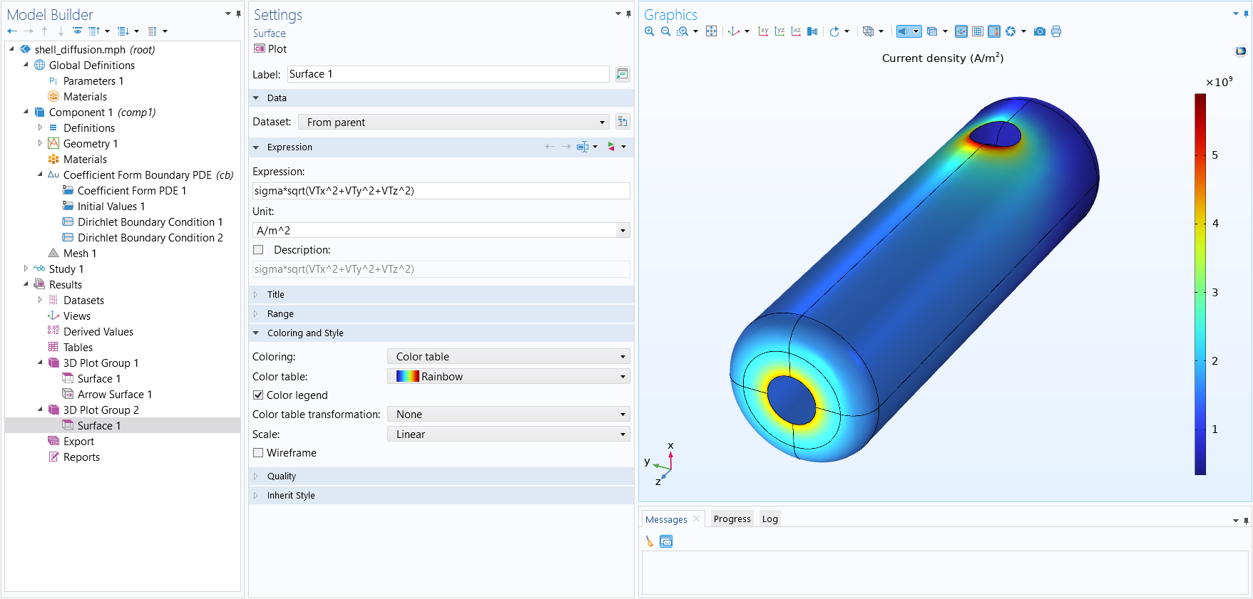 The Model Builder with the Surface plot selected, the corresponding settings, and the Graphics window showing the steel tank model in the Rainbow color table, with most of the model being blue.
The magnitude of the current density in the steel tank.
The Model Builder with the Surface plot selected, the corresponding settings, and the Graphics window showing the steel tank model in the Rainbow color table, with most of the model being blue.
The magnitude of the current density in the steel tank.
The model file for the steel tank example is available for download in the application library.
Coupling PDEs of Different Dimensions
We will now take another look at the tubular reactor tutorial model covered in Part 4 of this course. The model includes a lower-dimensional PDE on the exterior boundary. Since it is a 2D model, this PDE represents the cooling jacket of the reactor. In this case, the PDE describes the flow of the coolant and is a purely convective model. You can see the settings of the corresponding Coefficient Form Boundary PDE interface in the figure below.
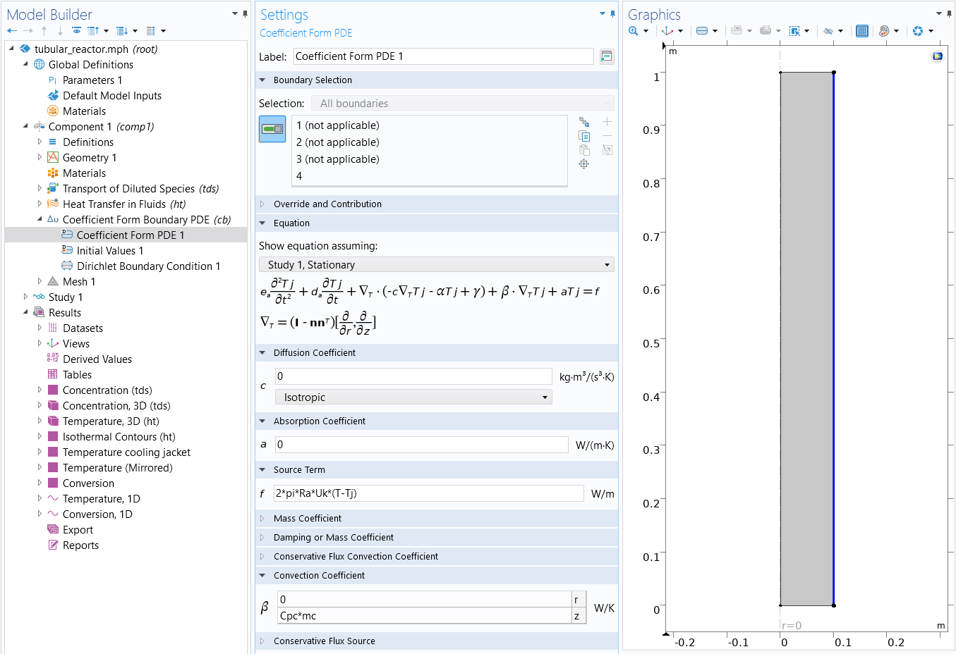 The Model Builder with the Coefficient Form PDE interface selected, the corresponding settings, and the Graphics window showing the tubular reactor model.
The Coefficient Form Boundary PDE interface for the tubular reactor model.
The Model Builder with the Coefficient Form PDE interface selected, the corresponding settings, and the Graphics window showing the tubular reactor model.
The Coefficient Form Boundary PDE interface for the tubular reactor model.
In the boundary equation, the dependent variable is Tj. At the same time, the dependent variable for the bulk domain of the reactor is T. They are coupled through the Source Term in this boundary PDE through the expression for f, 2*pi*Ra*Uk*(T-Tj). There is also an equal, though opposite, term in the Heat Flux definition of the Heat Transfer in Fluids interface equation that is used to model heat transfer in the bulk of the domain through the expression for the boundary flux qa: -Uk*(T-Tj).
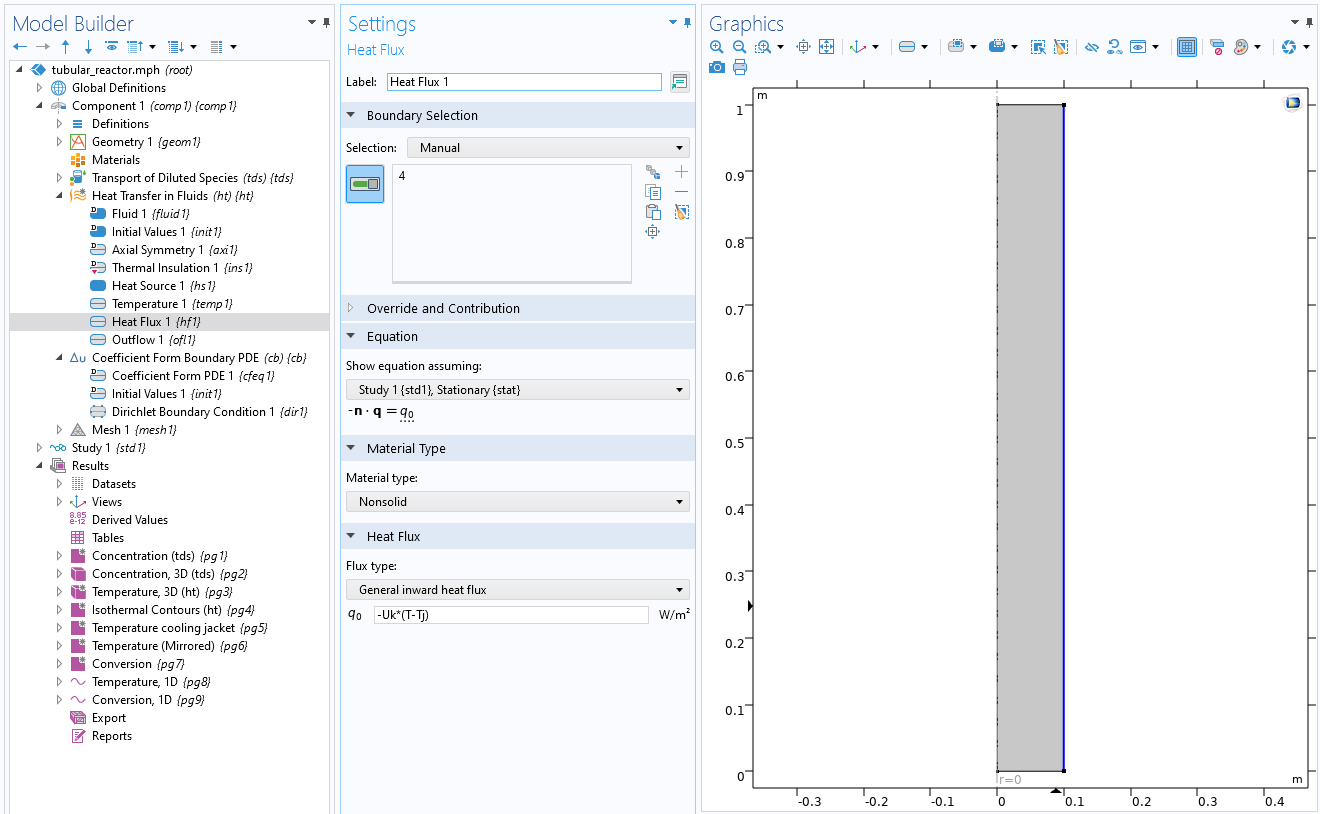 The Model Builder with Heat Flux selected, the corresponding Settings window, and the Graphics window showing the tubular reactor model.
The heat flux coupling linking the Coefficient Form Boundary PDE with the Heat Transfer in Fluids interface equation.
The Model Builder with Heat Flux selected, the corresponding Settings window, and the Graphics window showing the tubular reactor model.
The heat flux coupling linking the Coefficient Form Boundary PDE with the Heat Transfer in Fluids interface equation.
This is one example of how you can couple a lower-dimensional PDE with a PDE in an adjacent bulk domain. Using the Coefficient Form Boundary PDE notation, the boundary PDE can be written as:

with no diffusion coefficient:

but a source term:

where  is the radius of the reactor and
  is the overall heat transfer coefficient.
The convective part is:

where  and
and  are the heat capacity and mass flow rate of the coolant, respectively.
Modeling Distributed ODEs and DAEs
In the tubular reactor example, there was convection but no diffusion in the equation on the boundary. We can also have situations where there is neither diffusion nor convection. These situations usually occur when we have time-dependent equations. Going back to the Coefficient Form Boundary PDE:
the perhaps simplest case is when we have:

and all other coefficient set to zero.
This type of equation does not have any transport of information in the spatial direction since all the spatial derivative terms are zero. Instead, each point in space defines its own ODE. This type of equation is sometimes referred to as a distributed ODE or distributed state equation. It might, for example, represent some dynamic material property that only depends on the previous state of the material and not on the values in neighboring points. This type of equation is important enough that there are dedicated interfaces available in the Model Wizard, under ODE and DAE Interfaces, as shown in the figure below.
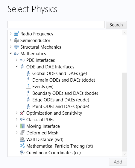
The Select Physics window, showing the available options under ODE and DAE Interfaces.
You can, of course, also have a system of distributed ODEs in two dependent variables, and  , such as:


You can define this type of system using the Domain ODEs and DAEs interface.
Now, if  , then the last equation is not actually an ODE but rather an algebraic equation. We have the system of equations:

This is called a differential-algebraic equation system. It turns up in many different application areas. COMSOL Multiphysics® can be used to solve such DAEs in many different contexts. Virtually all of the Mathematics interfaces can be used to define and solve such systems.
An important example of a PDE variant of this situation is when we have transient Joule heating:


where  and the other material properties can be functions of temperature and other field variables.
We can see that there are no time derivatives in the first equation, which represents the stationary current conservation equation. When solving this type of equation, COMSOL Multiphysics® uses a version of the so-called method of lines, which is capable of solving a DAE system. The first step taken by the assembly-solver machinery is to transform the PDE system into a system of DAEs. After that, specialized solvers that can handle systems of DAEs are used.
Modeling Distributed Algebraic Equations
Another degenerate case of a system of PDEs that we can have is when all the coefficients having derivatives are zero, for example:

This is a purely algebraic relationship and, just like for DAEs, virtually any of the Mathematics interfaces can be used to define and solve such systems. Whether you can solve it or not depends on if there is a solution, etc., as usual. Note that here, the dependent variables and are field quantities so that they can vary throughout space. The system can be made nonlinear, depending on the contents of the coefficients and source terms. For more information and an example of solving algebraic equations, see our blog post on solving algebraic field equations.
Field Continuity for Distributed ODEs and DAEs
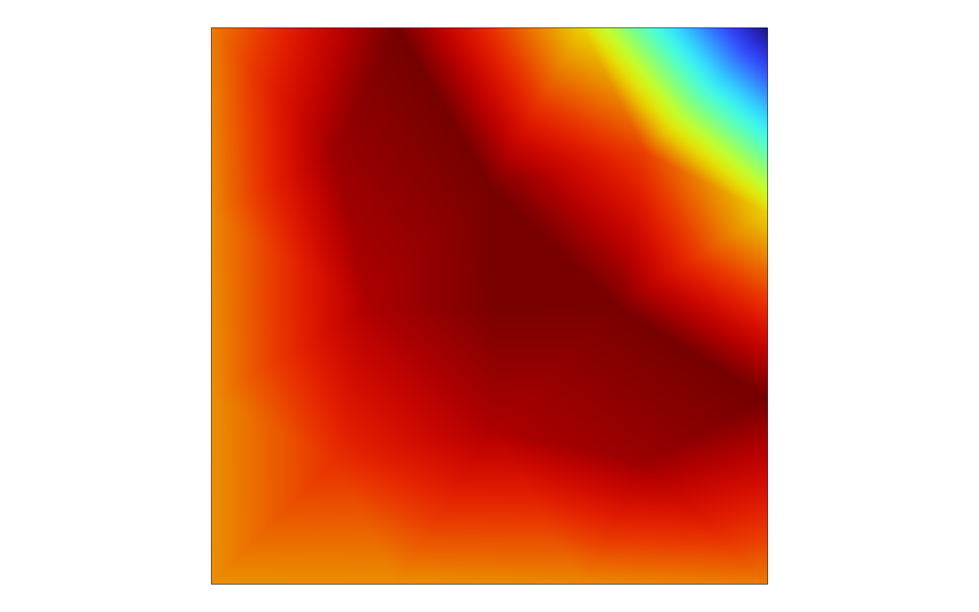
When solving for distributed ODEs and DAEs, including distributed algebraic equations, the equations are solved in a mean sense over the shape functions. Since, in this case, there are no spatial derivatives that link together the fields in neighboring shape functions, we can control the level of continuity in the fields by choosing different shape functions. The default setting in the Domain ODEs and DAEs interface is quadratic, or second-order, discontinuous Lagrange shape functions. This type of shape function allows a field variable to be discontinuous between elements. The images below show solutions to an equation solved using the Domain ODEs and DAEs interface with quadratic discontinuous Lagrange shape functions and quadratic continuous Lagrange shape functions. The discontinuous solution is approximated with a second-order polynomial within each element but has jumps between elements. The continuous solution is also approximated with a second-order polynomial within each element, but here, continuity is enforced between elements. Which option to choose depends on the physical interpretation of the field(s) that you are modeling.
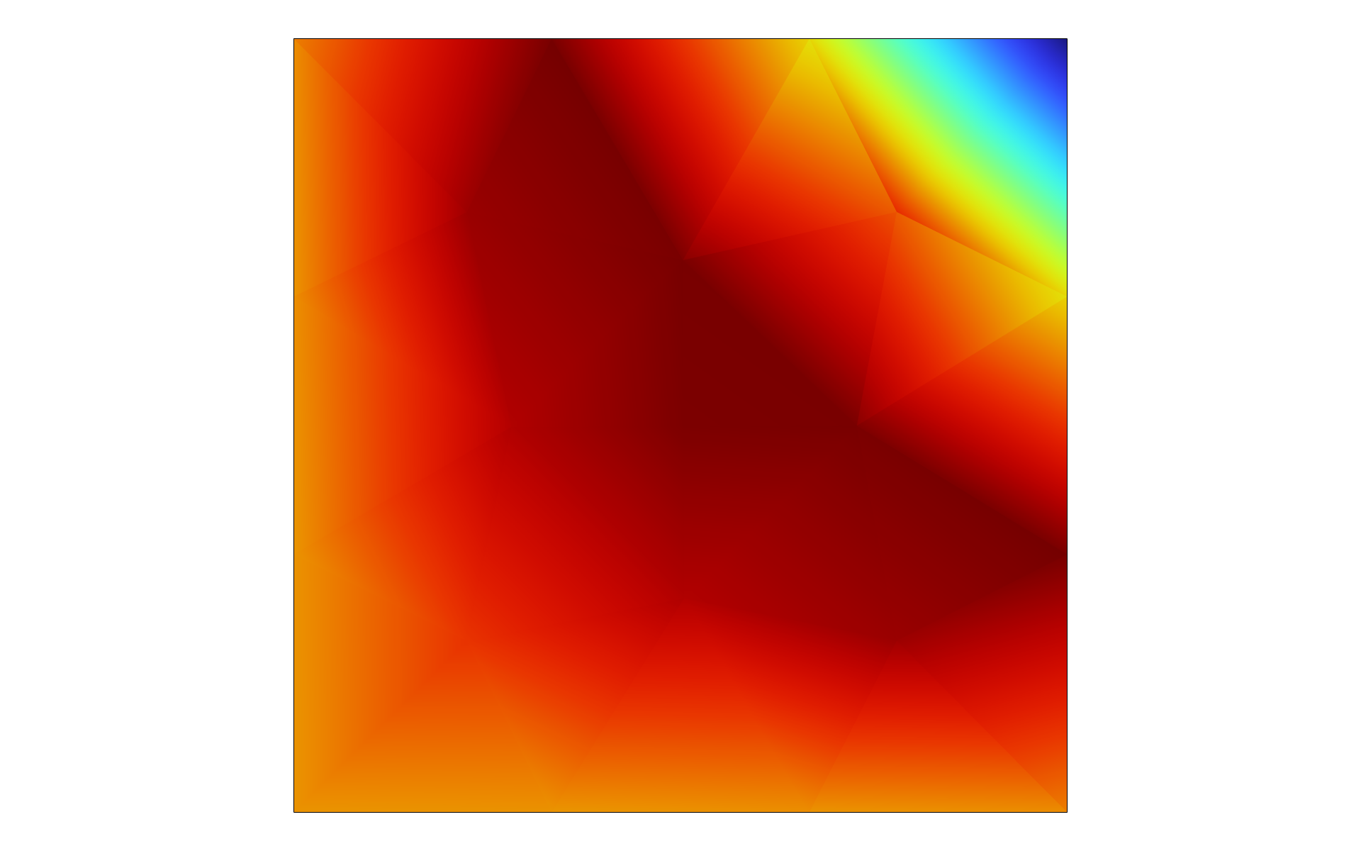
A solution to an equation using the Domain ODEs and DAEs interface with quadratic discontinuous Lagrange shape functions. A very coarse mesh is used to show the discontinuous jumps more clearly.
A solution to an equation using the Domain ODEs and DAEs interface with quadratic continuous Lagrange shape functions.
There are a number of other options for shape functions that could be useful, such as Gauss point shape functions. The important property of these shape functions is that they are completely independent from point to point, and are therefore suitable for solving local implicit material relations. When using these, one needs to take care in choosing the shape function order. This is so that it matches the integration point pattern of the other physics equations that are going to use the solution to the Domain ODEs and DAEs interface. When the point patterns match, the Gauss point shape function solution will, in practice, behave as if it were completely uncorrelated between any pair of points. It is only ever evaluated at the Gauss points. For more information on numerical integration and Gauss points, see our blog post "Introduction to Numerical Integration and Gauss Points".
Further Learning
Although the models used throughout this article are available for download, we encourage you to build the models yourself following the guidance provided in this article. This will help to reinforce how to set up PDEs in the software using the interfaces for Lower Dimensions. You can open and investigate the files for the model examples and compare them with implementation using the predefined physics interface.
Submit feedback about this page or contact support here.