Learning Center

Course:

Using Swept Meshes for Model Geometries

BACK TO LEARNING CENTER

How to Control the Swept Mesh

In the previous Learning Center article, we discussed the requirements for a geometry in COMSOL Multiphysics^® to be meshed using the Swept operation. In this article, we expand upon this by discussing how to obtain a quality swept mesh. What are the most important settings and considerations for generating a good quality swept mesh? We will address this question and more in this article. For our purposes here, we assume that each of the domains to be swept meshed are fulfilling every requirement discussed in the previous article.

Choosing the Source and Destination Faces

We learned in Part 2 that the direction of the sweep is important (because the software needs to be able to imprint the source faces over the destination faces). Does this mean that you need to manually make the selections for the source and destination faces? Not always; in the majority of cases, the source and destination faces are automatically detected by the software. The only cases when you would need to manually select the source or destination face is when the direction of the sweep is ambiguous: There are different paths that the sweep can take, and there may be one that is preferable, depending on the physics. This is especially true if you are meshing multiple domains in parallel; however, even in such a case it is usually sufficient to select the source faces, as COMSOL Multiphysics^® will automatically detect the destination faces based on the source faces you choose.

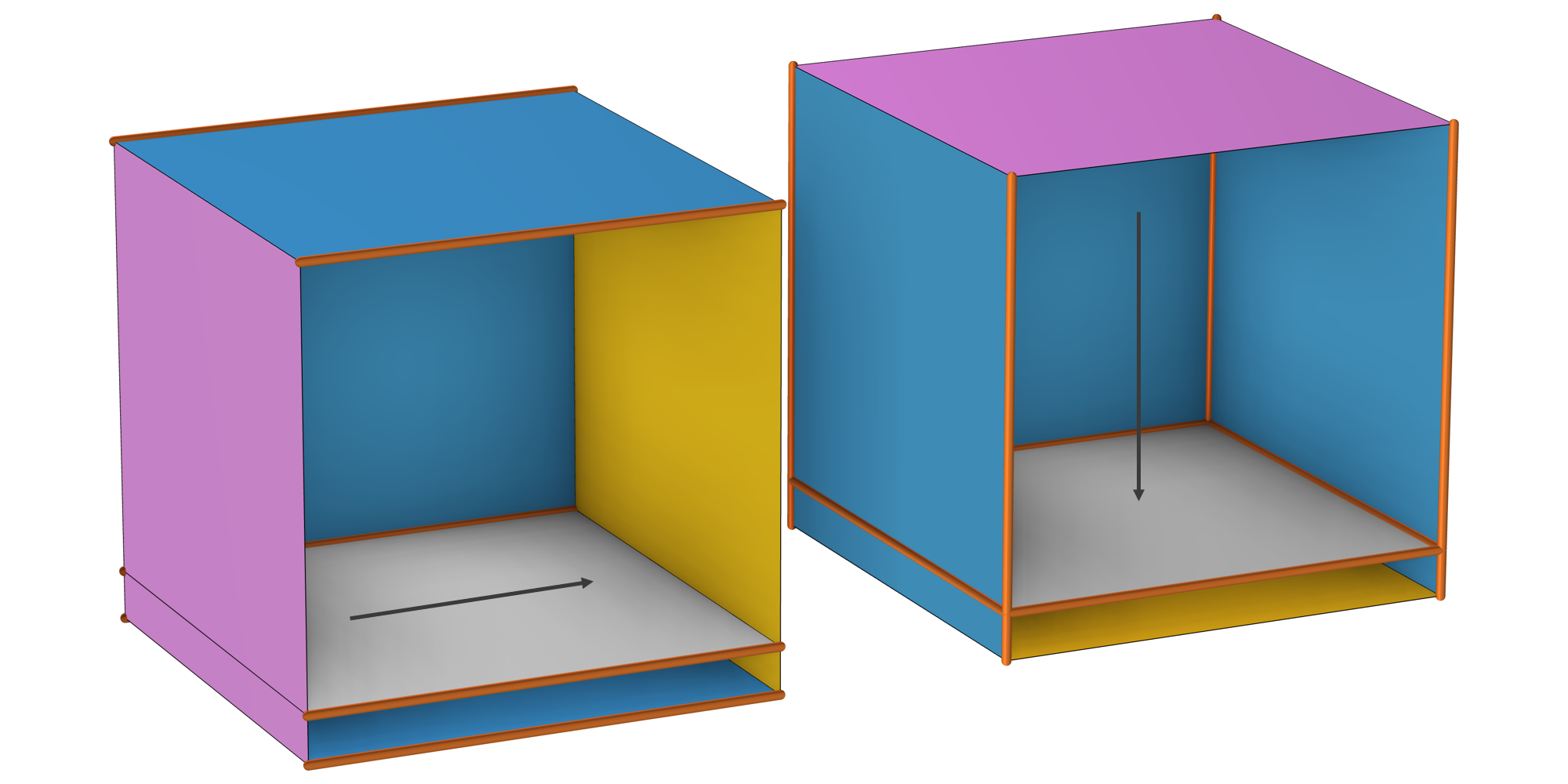
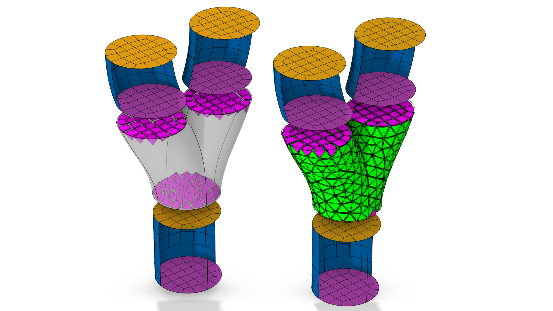
Two images of a block geometry with two arrows pointing in the different possible directions that a Swept mesh operation can take.

Two different sweep directions (indicated by the arrows). On the left, COMSOL Multiphysics^® has automatically picked the source face (in magenta) and the destination face (in orange) by default. In contrast, the image on the right shows a sweep performed with a user-defined source face, where COMSOL Multiphysics^® has automatically detected the destination face. (Front boundaries are hidden for visibility.)

The surface mesh is generated automatically by the Swept operation: The source face is meshed using a quadrilateral (i.e., quad) or triangular mesh, while the linking faces are meshed with a mapped mesh, and the destination face mesh is transferred from the source (via multiple methods, described in the documentation). In the following example, a triangular mesh is built on the source face.

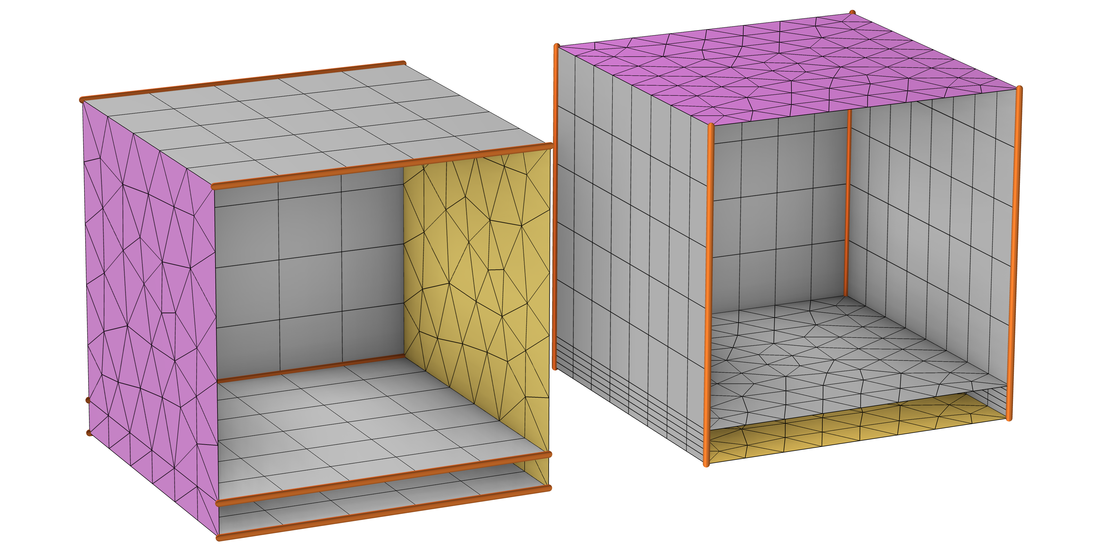
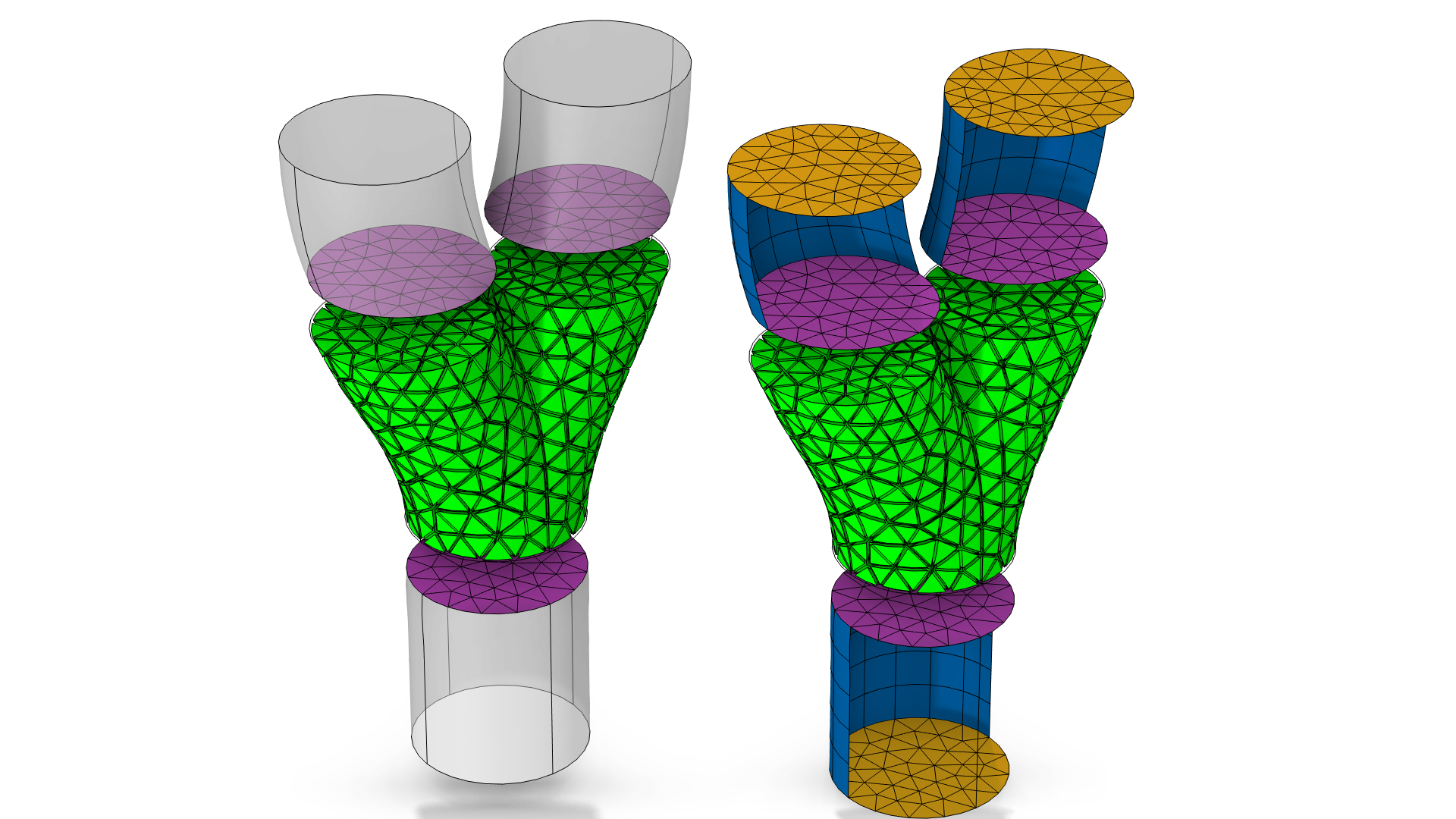
Two images of a block geometry meshed with different sweep directions; in the left image, the left face of the block is purple, and the right face of the block is orange. In the right image, the top face of the block is purple, and the bottom face of the block is orange.

The resulting surface meshes for the two sweeps depicted above. (Front boundaries hidden; linking face meshes depicted by the gray grids.) Because the source face was user defined for the swept mesh on the left and detected by the software for the mesh on the right, two different meshes were generated. Note that a Distribution subnode acts along the sweep direction in both cases. Depending on the physics, one mesh might be preferable to the other.

There is also the option to manually generate the surface mesh for the source face first, after which you would add a Swept mesh operation, which is explained more below.

Controlling the Mesh Size and Distribution

As explained in more detail in our blog post on meshing domains with different size settings, it is a good practice to use one mesh operation with many local size attributes instead of repeating several mesh operations. This also relates to the parallelization of the meshing algorithm. The Swept operation is no exception to this rule, so let's have a look at the two attributes that are available. To add an attribute, right-click the Swept node and select Size or Distribution.

Size

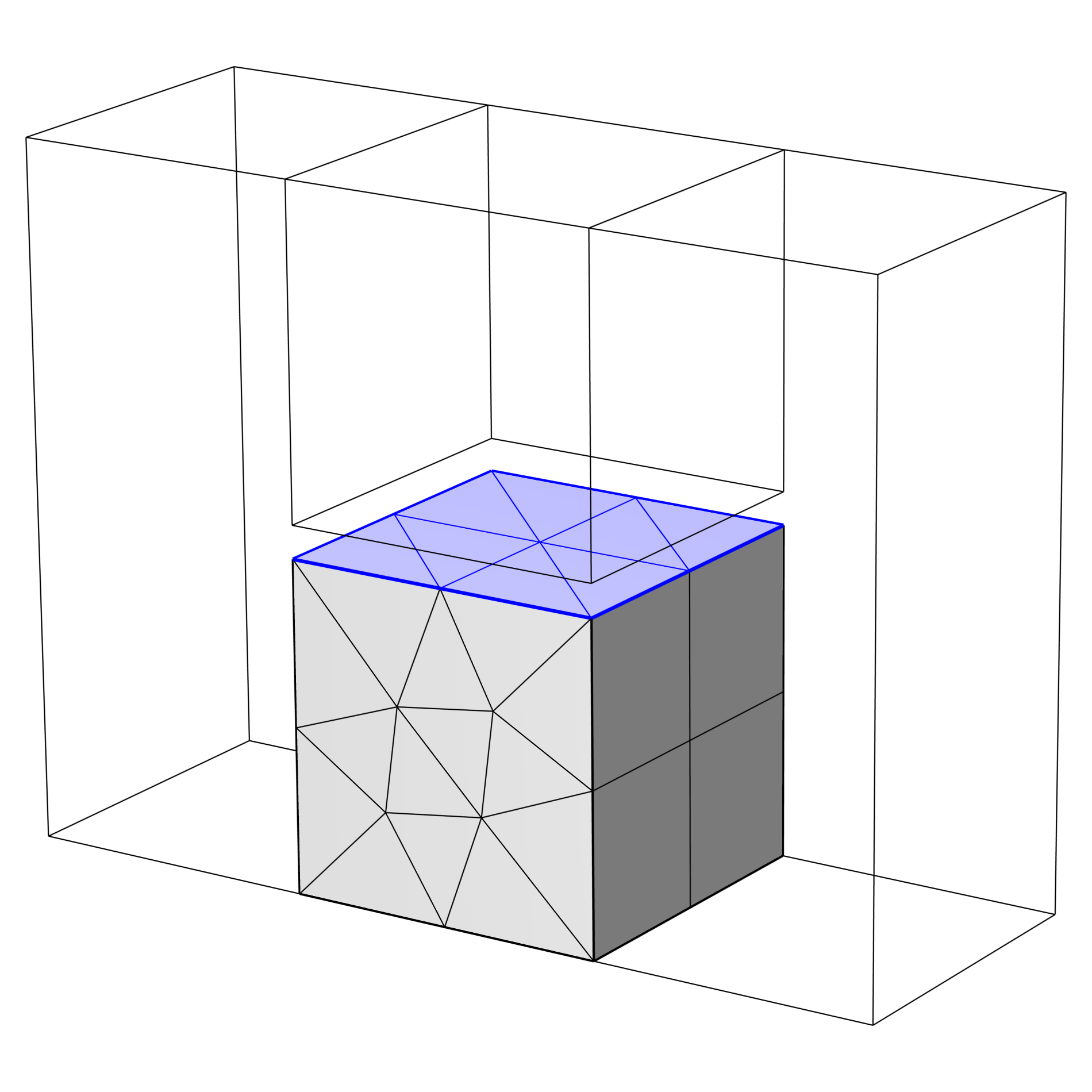
You can use a Size node for setting up a maximum or minimum element size in the domains or on the boundary level for the source faces. The maximum or minimum size expressions can be dependent on physics variables, parameters, or expressions that include variables and parameters. If you want to control the size on the source faces, make sure to set the same boundaries as source faces for the Swept node. See also the section "When and How to Premesh the Source Faces" below.

The boundaries of a heating element are selected in blue. Adding a Size attribute to control the element size on the selected (blue) boundaries of this heating circuit.

Distribution

For Swept, the Distribution attribute specifies how many mesh element layers there are along the sweep direction. If you want to control the distribution along an edge, you need to premesh a boundary or edge, as explained below. The result is determined by the Distribution Type and the associated settings. If a similar element size is wanted in several domains, consider using a Size attribute instead.

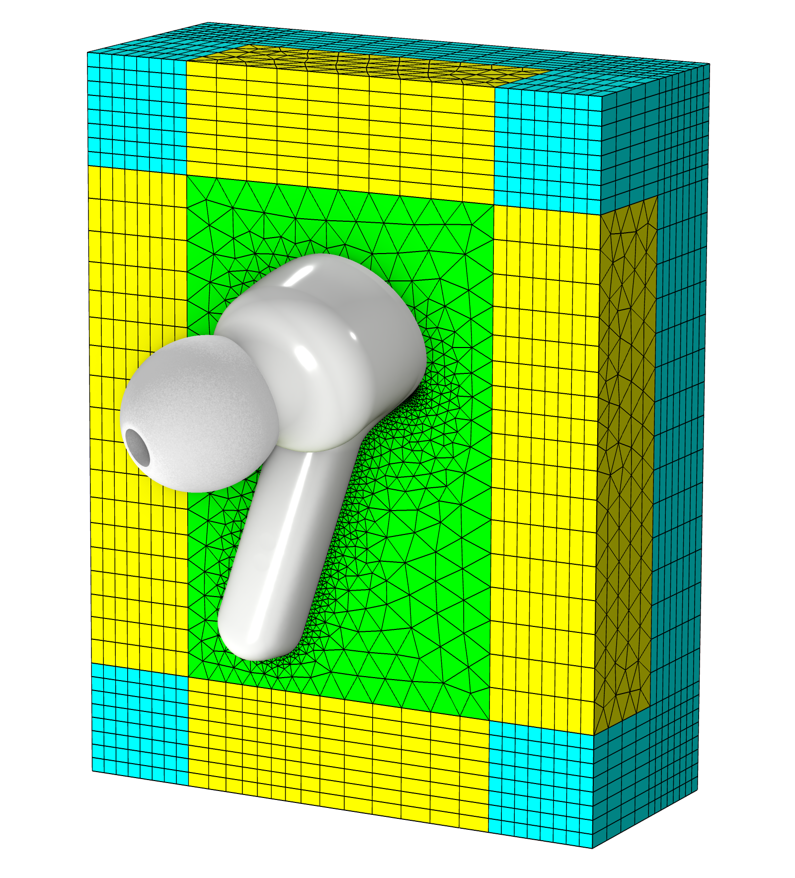
A simulation of the acoustic domains surrounding an ear bud. Domains are distinguished blue, green and yellow colors corresponding to different mesh sizes and shapes.

A typical example where the Distribution node is used. An acoustics simulation of an ear bud where the outermost domains are defined using a Perfectly Matched Layer node with a specification of eight elements in the sweep direction (yellow and cyan).

The default Distribution type is Fixed number of elements. Change this setting to Predefined to specify an element distribution that is either linearly or exponentially growing. This helps to obtain a smooth size transition between adjacent domain, required by some physics, such as in fluid mechanics.

When setting up any predefined distribution, the number of elements and the element ratio (ratio between the largest height and the smallest height ) are the input numbers:

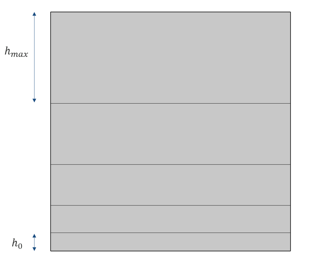A graph shows the lengths of the domains in an asymmetric distribution.

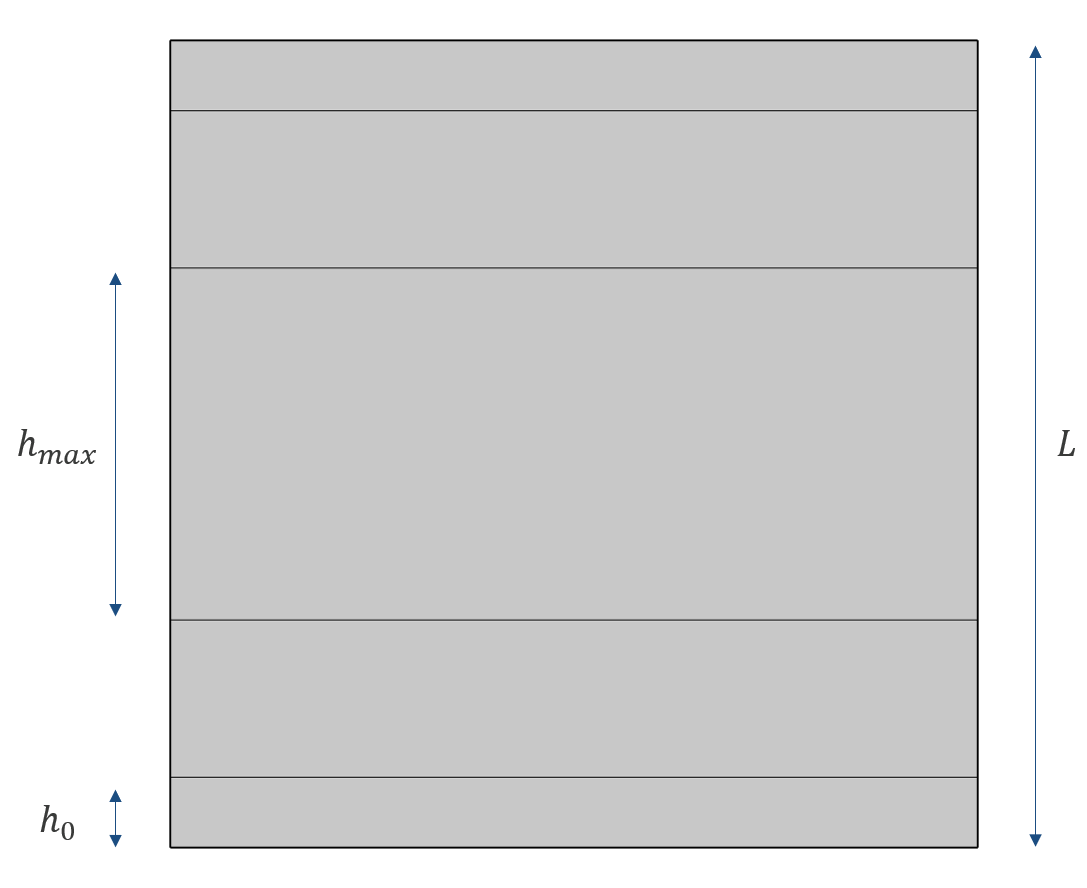A graph shows the lengths of the domains in a symmetric distribution.

Definition of the different lengths for an asymmetric (left) and symmetric (right) distribution. The total length is noted as .

While, most of the time, the parameters can be tweaked manually so that the mesh is satisfactory, one might want to have more control of the mesh growth rate. In the table below, some useful relations for the asymmetric distributions are presented. The symmetric distributions depend on the parity of , but are approximated (equal when is even) if and are replaced by and , respectively.

Expression	Linear	Exponential

It might be the case that and the maximum local growth rate, , between consecutive heights () are known.

Let's say, for example, that you want to be equal to the size of the mesh on the cross section, and that the maximum growth rate is fixed by the global size node. How do you deduce and ? Let us find out with an exponential distribution.

Generally, the height is bounded, so that . The first step is to ensure this is true even when . (The goal is to use the least amount of elements.) Consequently, from the last line of the table:
From here, and are deduced by rearranging the third line and by definition of :
Finally, using the second line, can be approximated as the closest integer to .

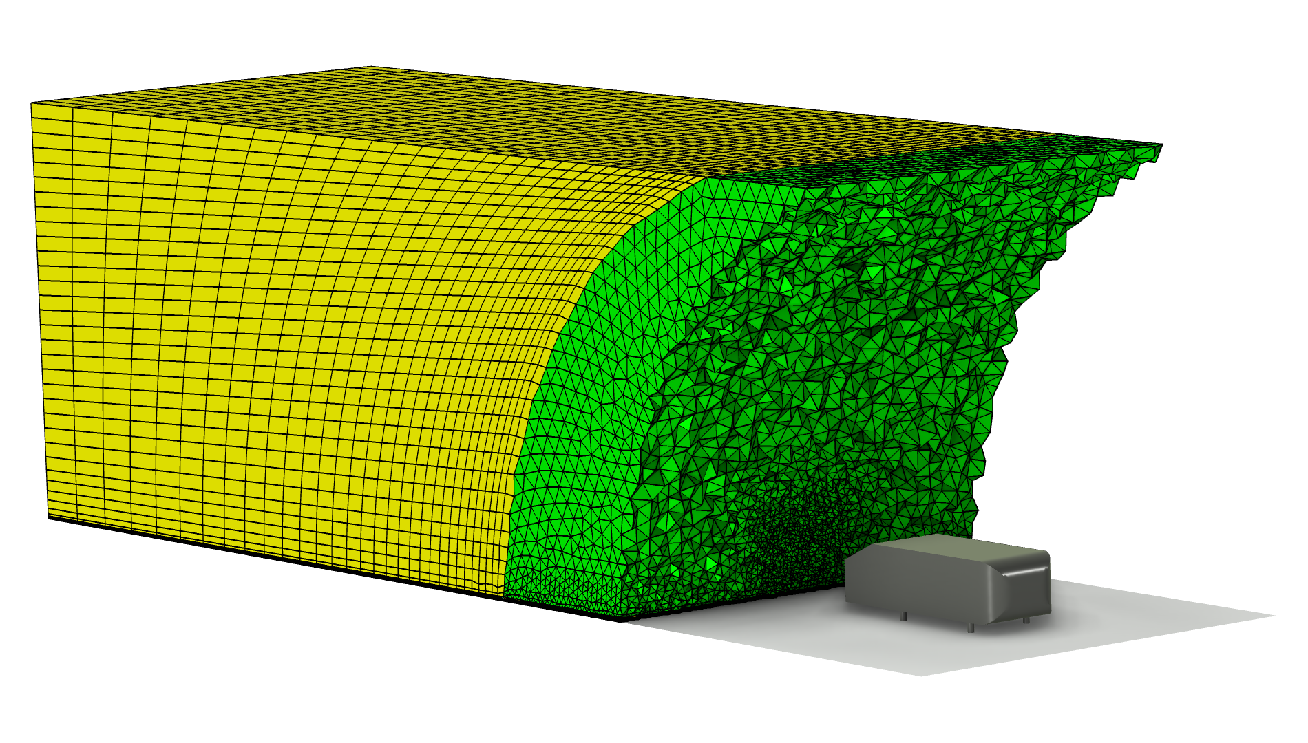The mesh for the fluid flow domain surrounding an Ahmed body, where the coarser mesh that's farther from the body is yellow and the finer mesh that's closer to the body is green. The Swept mesh (in yellow) behind the Ahmed body has been modified to make use of the exponential distribution in order to smoothly increase the size of the mesh elements.

Adding a boundary layer mesh can sometimes be an alternative to using a predefined distribution in the sweep. This is shown below with the pictured example.

Two side-by-side figures of the Steam Reformer tutorial model geometry showing the inserted boundary layer mesh highlighted in blue on the right.

The Steam Reformer tutorial model geometry. Here, a boundary layer mesh is added at the beginning of the geometry, instead of a symmetric distribution. The inserted boundary layer mesh elements are highlighted in blue.

There is also the option to manually generate the surface mesh for the source face first, and then follow this with adding a Swept mesh operation. Doing so enables you to use mesh operations (e.g. Size and Distribution subnodes) to achieve a desired face meshing on the source face, which you can then sweep into a 3D mesh. Examples of which can be seen here.

When and How to Premesh the Source Faces

Although the surface meshing for a domain can be handled automatically using the Swept operation, there are cases in which you will want to premesh the source faces to have more control over the mesh on those boundaries. By premesh, we mean meshed by a previous operation.

It is important to note that any faces already meshed prior to adding a Swept operation will automatically be selected as the source faces, unless meshed with a mapped mesh where they can also be used as linking faces. You can use a Free Quad, Free Triangular, or Mapped operation to premesh the source faces when needed (examples of which can be seen here.) Some use cases for premeshing the source faces include when you need:

A boundary layer mesh. For a swept mesh, it is recommended to add the boundary layers on the source faces before it is swept. (See the below image.)
A Distribution attribute to control the edge mesh on the source faces.
A mapped mesh on the source faces.

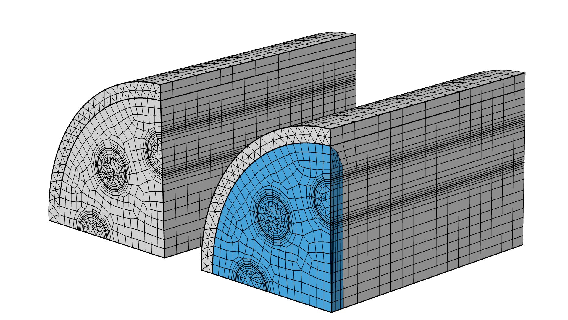
Three side-by-side figures of the Steam Reformer tutorial model geometry showing the boundary layer mesh. The Steam Reformer tutorial model geometry. The boundary layer mesh is added to the source faces first.

Note: If multiple faces are meshed prior to the Swept operation, make sure that: 1. The linking faces are meshed using a Mapped operation. 2. The destination mesh precisely matches the source.

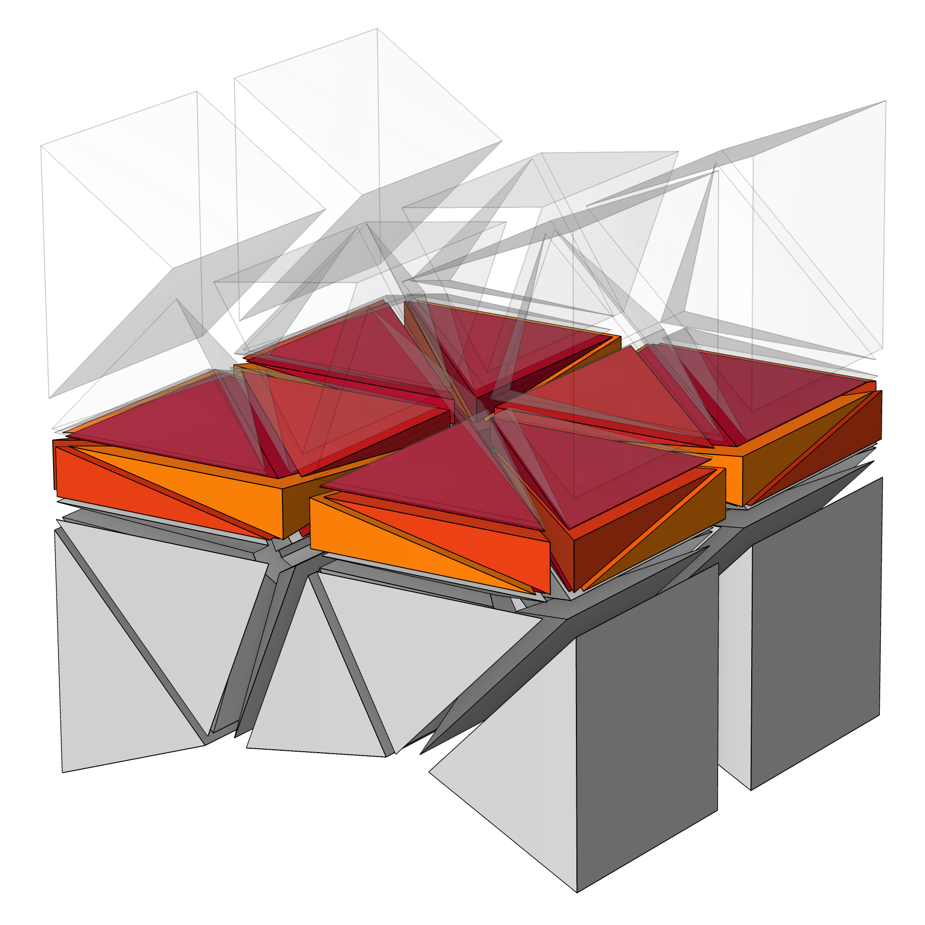
Premeshing edges can also be useful. For example, if varying curvature is important for your model and you want to have more control of the distribution, mesh some edges before the Swept operation. The Edge operation can take the curvature factor into account while maintaining a continuous growth rate change.

The image on the left depicts the mean curvature of a geometry to be meshed. To account for the curvature, the top chain of edges is meshed first in the center image. The Edge operation can itself have several size attributes. In this example, the top curve has a curvature factor of 0.1, while the bottom one has a curvature factor of 0.2. The sweep shows the mesh size changing incrementally across the domains to create a smooth transition in the image on the right.

Consideration of the Adjacent Domains

Any domain adjacent to the one where the mesh is swept can either be meshed before or after the sweep. If an adjacent domain is meshed before the sweep, the face meshes can be considered to be premeshed.

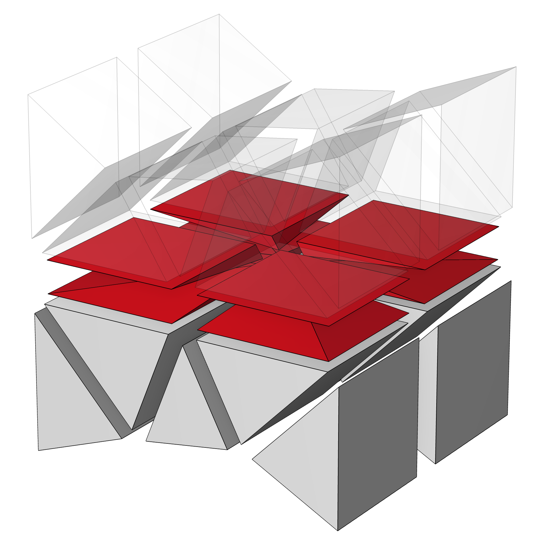
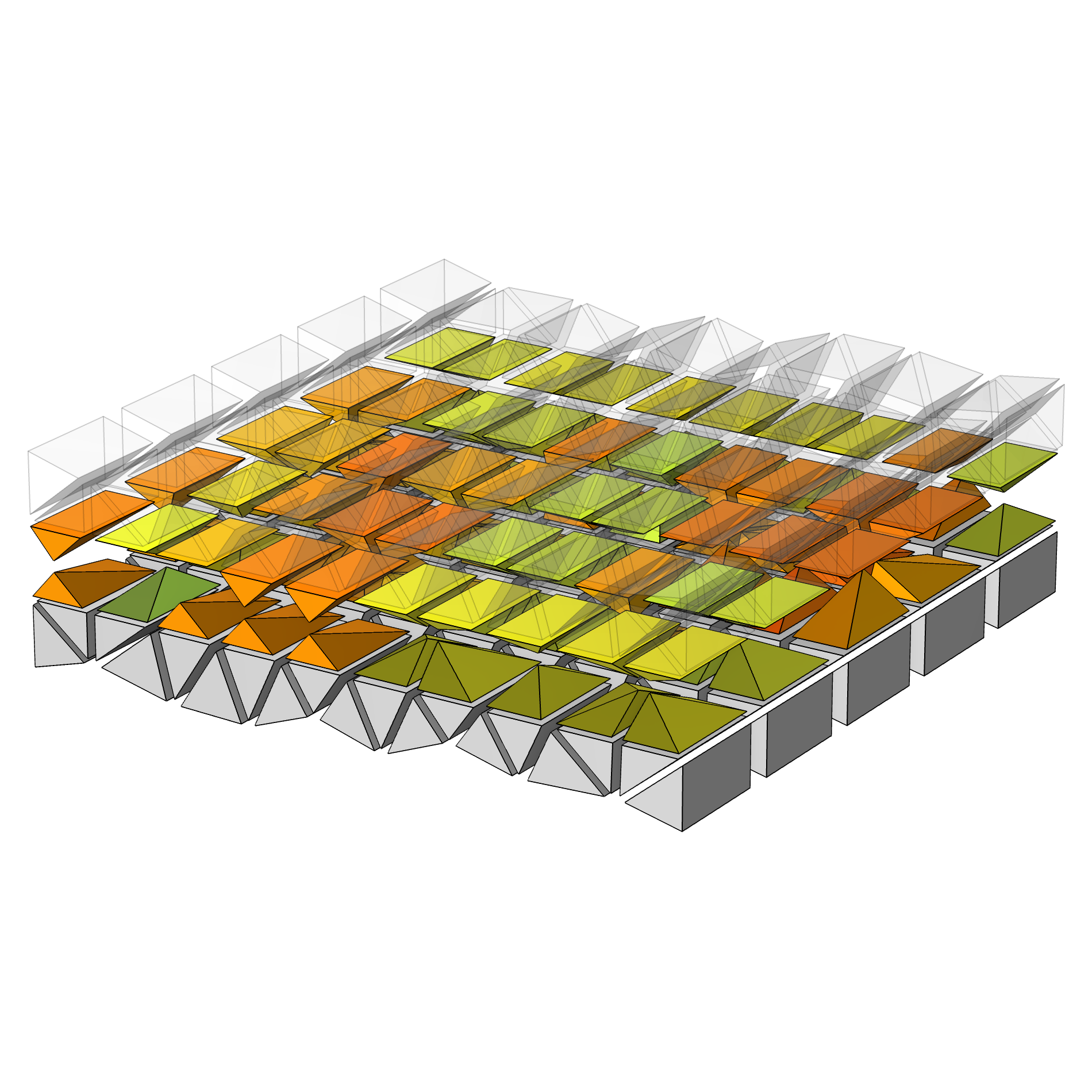
The Y-shaped geometry from part 2, but here the automatic face meshing method has been used. Notice the difference between building the Swept node before the Free Tetrahedral node (left) and building Free Tetrahedral before Swept (right). Pyramids (magenta) are inserted to match the quad mesh of the swept domains (left) as opposed to the triangles from the tetrahedral elements (green) are used as a source mesh for Swept (right).

If the domain is already swept, a mapped mesh is generated on the linking faces. A layer of pyramids (magenta in the animation below) are inserted closest to the linking faces which enables a transition between the swept mesh elements (yellow quads) and the tetrahedral mesh elements (i.e., green volume mesh elements with only triangular mesh faces) in the surrounding domain. See [this blog post](https://www.comsol.com/blogs/how-to-inspect-your-mesh-in-comsol-multiphysics](https://www.comsol.com/blogs/how-to-inspect-your-mesh-in-comsol-multiphysics) for information about creating mesh plots.

In the carbon fibers tutorial, the fibers are first swept meshed before the surrounding domain is filled by a Free Tetrahedral mesh; pyramids are inserted automatically to connect the two mesh types. For visualization purposes, the front tetrahedra are hidden.

Depending on the number of layers that are inserted along a sweep, the pyramids can become very elongated in one direction which, for some physics, should be avoided.

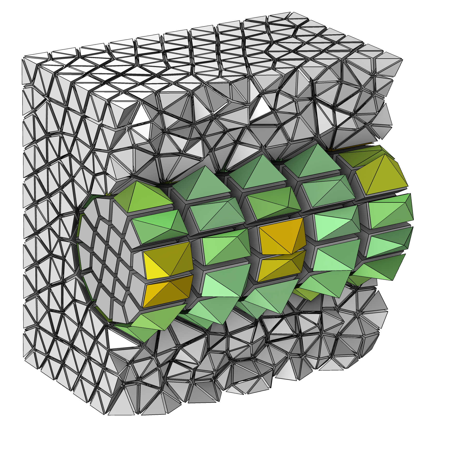A swept meshed cylinder with five element layers, with the skewness quality depicted as green pyramids with relatively high peaks.

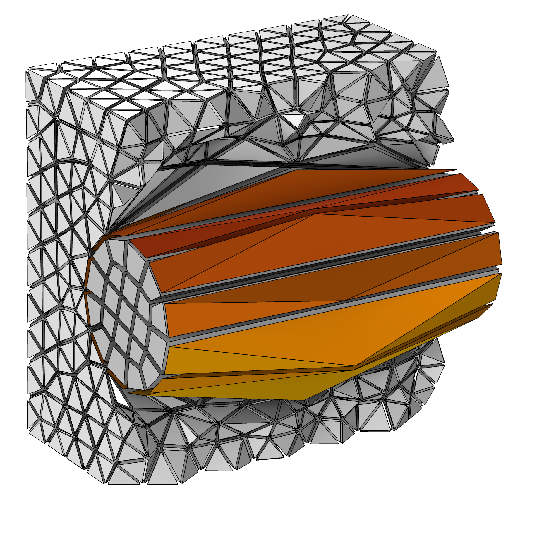A swept meshed cylinder with one element layer, with the skewness quality depicted as flat orange pyramids.

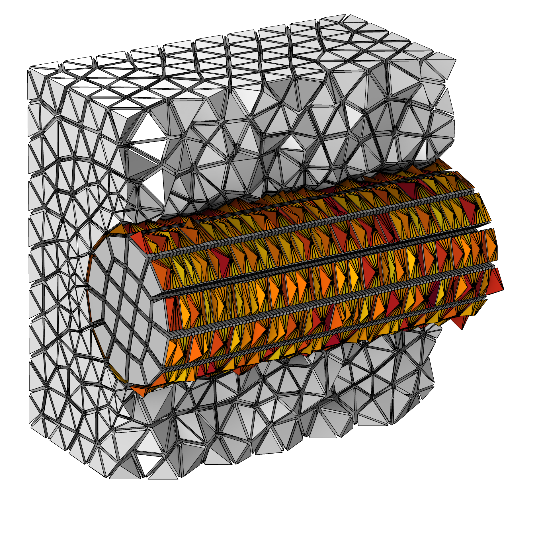A swept meshed cylinder with 100 element layers, with the skewness quality depicted as small orange pyramids.

A cylinder is swept meshed with five element layers on the left), only one in the middle, and 100 on the right. A light green color indicates a pyramid with similar base and height lengths while an orange/red color indicates a pyramid that is very stretched in one direction.

Things to consider, in case an inserted pyramid becomes too elongated.

Change the distribution of the elements along the sweep so that the quads have more similar side lengths.
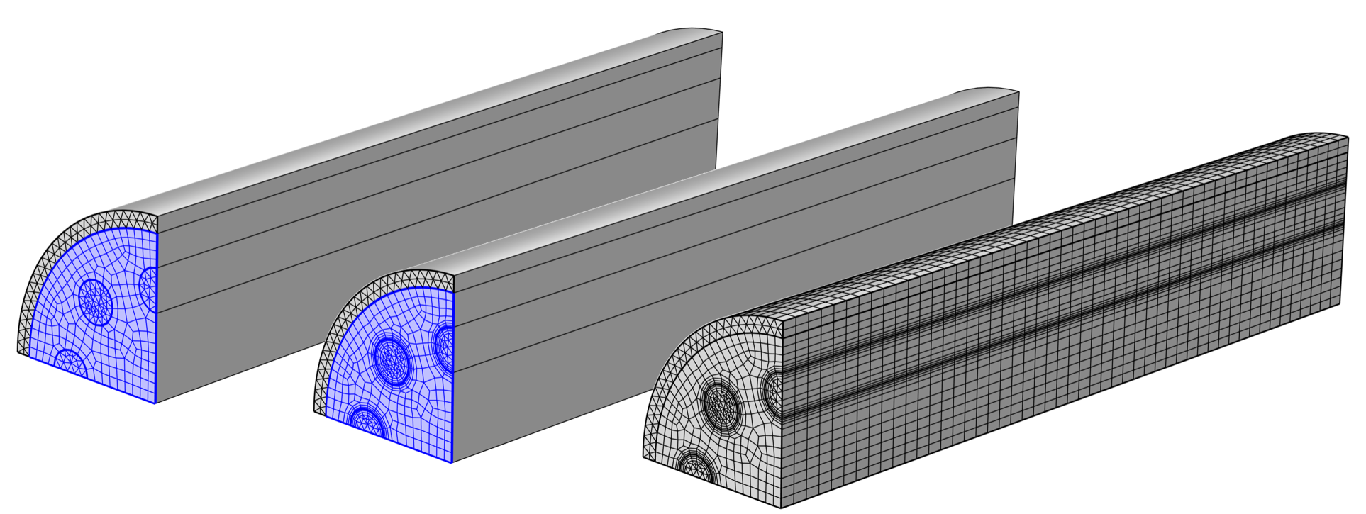
Premesh the source faces. Set a size setting or distribution such that the mesh along the outer edges better matches the distribution of element layers in the sweep. Compare the two first sets of images below.
Include the surrounding domains in the sweep, if possible. There might be a need to partition adjacent domains for this to work.
Use the Form an Assembly action to finalize the geometry. See the following article for more information.

Note that the physics may also set requirements on the mesh. This is not taken into account here.

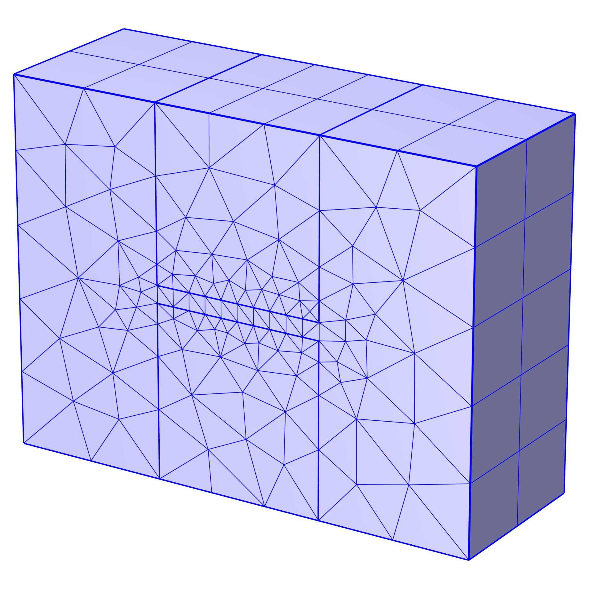
Even if you take care that the quads have similar side lengths, there are also some things to consider when the adjacent domain has a thin domain region.

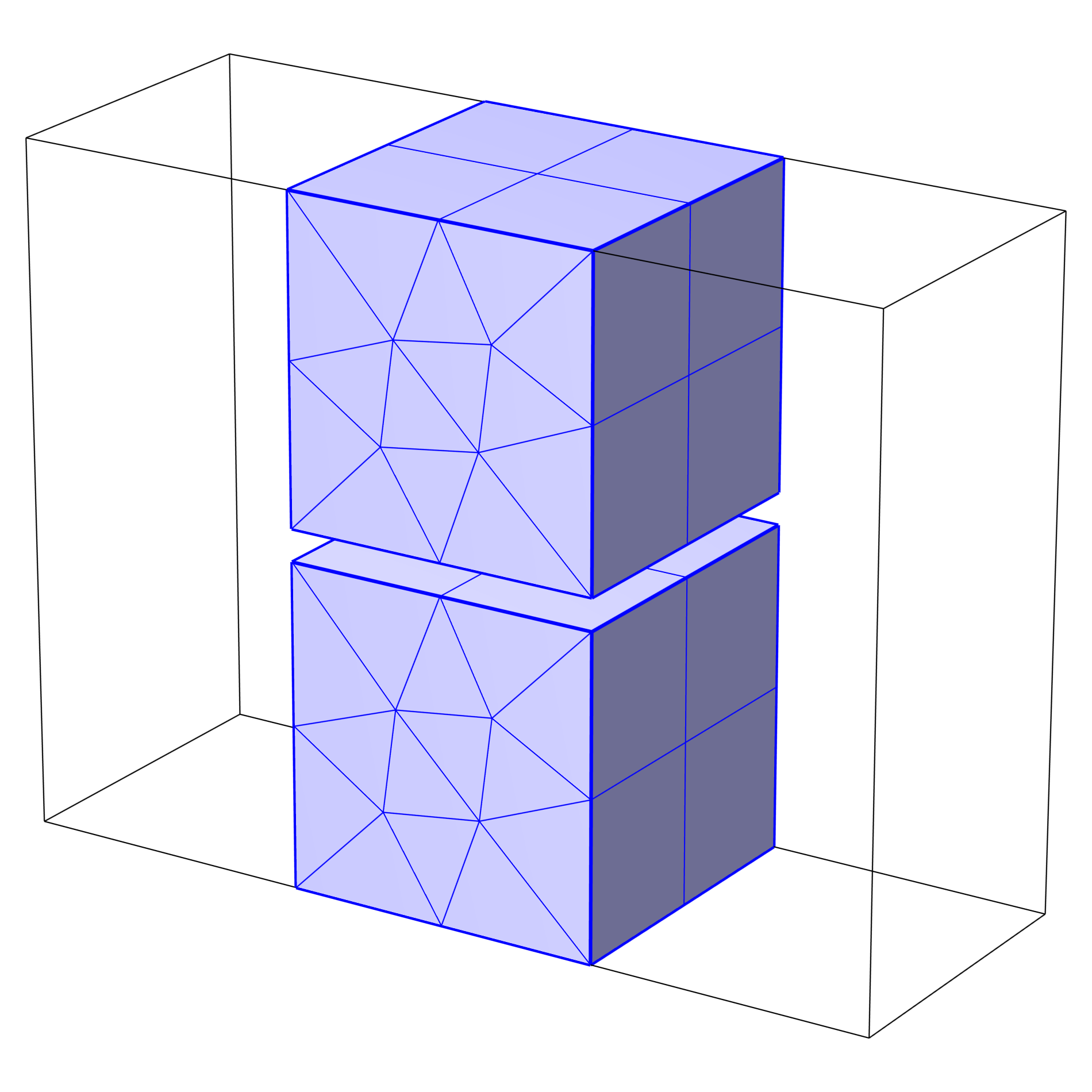Two identical meshed cubic geometries, one above the other with a thin space between.

A close-up of the meshed space between the two blocks, showing low quality, flat pyramids.

Inserting pyramids in a narrow domain region adjacent to domains with a swept mesh. Although the quads have equal side lengths, the pyramids become flat due to the thin domain region, as is indicated by the red color. (Only the pyramids and hexahedra near the narrow domain region are shown.)

If the thin domain represents a thin layer, consider if it is possible to use a boundary condition rather than modeling the thin layer explicitly. An example of this is explained in this blog post . If it is not relevant for the physics, consider collapsing the narrow region using geometric operations.

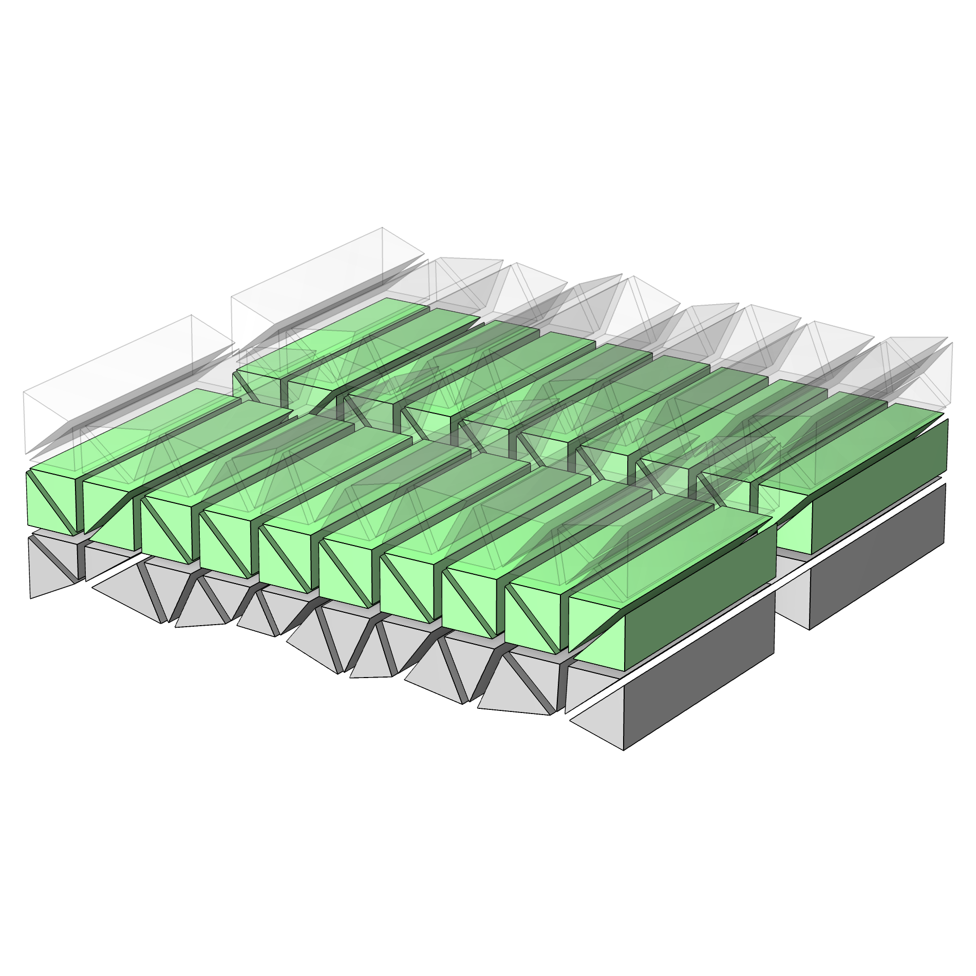
If the thin domain region must be included, one solution is to refine the mesh size on the source faces close to the narrow domain region and increase the number of element layers so that the size of the quads become more equal to the thickness of the region. This will result in more mesh elements in total, compared to the earlier cases.

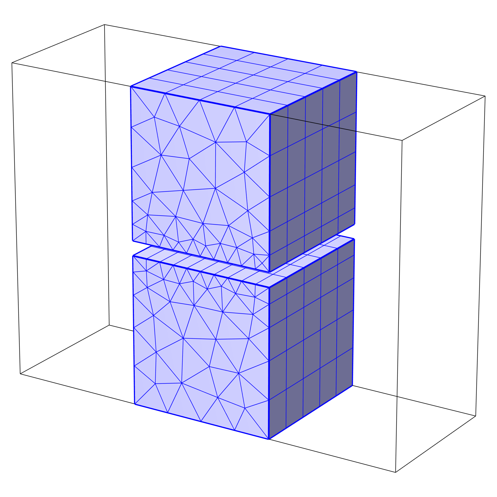A thin layer of space between two vertically stacked blocks is meshed with a refined size.

A close-up of the meshed space between two stacked blocks, showing an increased number of mesh elements.

Premeshing the source faces of the sweep with a finer size setting near the narrow domain region. The image to the right shows that the pyramids are less flat compared to before.

This technique can sometimes require a lot of mesh elements in order to correctly resolve the gap.

In this example geometry, it is also possible to sweep all domains together in one Swept operation. It is also possible to partition the H-shaped domain so that the narrow domain region becomes its own domain (this will give 5 domains in this geometry). This is not shown.

A mesh of several cubic domains all swept together, with prism and hexahedron mesh elements.

A close-up of the hexahedron mesh of the thin domain included in a sweep of several cubic domains.

In this swept mesh, no pyramid elements need to be inserted.

Finally, in some cases it can help to first convert the quads using the Convert operation. By converting the quad elements, no pyramids need to be inserted. However, this also splits some of the elements in the swept mesh. With this in mind, make sure you monitor the mesh quality.

Triangular mesh elements of a thin domain between two stacked blocks, with the top block hidden for visibility.

A close-up of the low quality tetrahedra that result from converting the mesh elements of a thin domain between two stacked blocks from quad to triangular.

The faces near the narrow domain region are converted from quads to triangles. (The mesh from the top cube is hidden in the left image.) This means that no pyramids have to be inserted into the thin region, although it is important that the converted quads are of similar size to the thickness of the region not to get too anisotropic tetrahedrons.

Further Learning

Several examples were depicted in this article that complemented our discussion on the most important aspects to take into account so that a swept mesh of good quality can be generated. You can find the MPH files for these examples attached to this article and see firsthand for yourself how this was accomplished for several types of geometries.

Submit feedback about this page or contact support here.