Solving Multiphysics Problems

Here we introduce the two classes of algorithms used to solve multiphysics finite element problems in COMSOL Multiphysics. So far, we’ve learned how to mesh and solve linear and nonlinear single-physics finite element problems, but have not yet considered what happens when there are multiple different interdependent physics being solved within the same domain.

A Simple Steady-State Multiphysics Problem

Let’s start by considering a very simple steady-state multiphysics problem: A coupling of steady-state electric current flow through a metal busbar, heat transfer in the bar, and structural deformations. Resistive heating arises due to the current flow, which raises the temperature of the bar and causes it to expand. In addition, the temperature rise will be significant enough that the electrical, thermal, and structural material property variations with temperature must be considered. We want to find the current flow, temperature fields, and deformations and stresses under steady-state conditions. The figure below shows a schematic of the problem being solved.

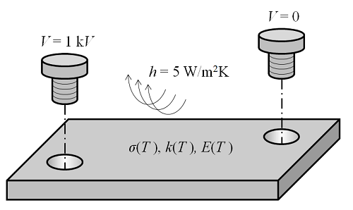
The multiphysics problem at hand.

The Associated Equations

There are here three governing partial differential equations being solved. First off, the equation that describes the voltage distribution within the domain is:

After discretizing via the finite element method, we can write a system of equations as:

where the subscript, _{V}, denotes the voltage unknowns, and the system matrix, \mathbf{K}_V, is dependent upon the temperature unknowns, \mathbf{u}_T. Assuming that the voltage distribution is known, then the volumetric resistive heating can be computed from:

where \bf{E}, the electric field, is: -\nabla V. This heat source shows up in the governing equation for temperature:

And this equation gives us the system of equations:

Once we have the temperature distribution within the domain, we can solve for the structural displacements:

where the elasticity matrix, \bf{C}, is computed based on the temperature-dependent Young’s Modulus, E(T). The imposed thermal strain is \epsilon_{\Delta T} = \alpha(T-T_0) and the strain is \epsilon = 1/2 [{\nabla \mathbf{u}^\mathbf{T}_D + \nabla \mathbf{u}_D}]. The system of equations that solve for the displacements is written as:

where the subscript, {_D}, indicates the displacement unknowns.

We can combine these systems of equations together:

For brevity, we can omit subscripts in the arguments:

That is really all there is to it! There is no conceptual difference at all between solving a single-physics nonlinear problem and solving a coupled physics problem. Everything that we have already learned about solving nonlinear single-physics problems, including all of the discussions about damping, load and nonlinearity ramping, as well as meshing, is just as valid for solving a multiphysics problem.

Fully Coupled Approach

But it is also important to understand a (sometimes very serious) drawback to the above approach. During the Newton-Raphson iteration, we need to evaluate the derivative, \mathbf{f'(u}^{i}), so let’s write that out:

where we use a shorthand notation to simplify and to compact the expression of the derivative, e.g.:

Clearly, the above matrix is non-symmetric, and this can lead to a problem: If the system matrix is not definite, then we may need to use the more memory-intensive direct solvers. (Although iterative solvers, with the right choice of preconditioner, can solve a wider class of problems they cannot be guaranteed to handle all cases.) Solving such a multiphysics problem with a direct solver will be both memory- and time-intensive.

However, there is an alternative. The above method, called a Fully Coupled approach, assumes that all of the couplings between the physics must be considered at the same time. In fact, for the purposes of solving many types of multiphysics problems, we can neglect these off-diagonal terms during the solution, and solve using a more memory- and time-efficient Segregated approach.

Segregated Approach

The Segregated approach treats each physics sequentially, using the results of the previously solved physics to evaluate the loads and material properties for the next physics being solved. So, using the above example, we first take a Newton-Raphson iteration for the voltage solution:

where, for the first iteration, we must have a starting guess for voltage and temperature ( \mathbf{u}_V^{i=0} , \mathbf{u}_T^{i=0} ). The material properties are evaluated using the initial conditions given for the temperature field. Next, the temperature solution is evaluated:

where, for the first iteration, i=0, the initial conditions given for the temperature field are used to evaluate the materials properties, \mathbf{K}_T(\mathbf{u}_T^{i=0}) , but the loads are evaluated based upon the voltage solution that was just computed: \mathbf{b}_T(\mathbf{u}_V^{i=1}) . Similarly, the displacement field is solved:

where the material properties and loads for the structural problem are computed using the temperature field computed above.

These iterations are then continued: voltage, temperature, and displacement are repeatedly computed in sequence. The algorithm is continued until convergence is achieved, as defined earlier.

The great advantage to the above approach is that the optimal iterative solver can be used in each linear substep. Not only are you now solving a smaller problem in each substep, but you can also use a solver that is more memory-efficient and generally solves faster. Although the segregated approach generally does require more iterations until convergence, each iteration takes significantly less time than one iteration of the fully coupled approach.

The algorithm used by the segregated solver for a model composed of n number of different physics is:

1. Choose initial conditions for all physics in the model
2. Initialize a counter for the number of iterations
3. Solve for the first physics in the segregated sequence, using the previous step to evaluate material properties
4. Solve for the second physics, using the part of the solution that has been computed to this point
5. …
6. Solve for the n^th physics, using the (n -1)^th previously computed parts of the solutions
7. Repeat 2-6 until convergence, or until the desired peak number of iterations is exceeded

For general multiphysics problems, you will still have to choose the order in which the physics are solved, but the software has default suggestions as to an appropriate sequence for all built-in multiphysics interfaces. COMSOL Multiphysics will provide default linear solver settings for each physics in the segregated sequence.

When the segregated approach is applicable, it will converge to the same answer as the fully coupled approach. The segregated approach will usually take more iterations to converge; however, the memory and time requirements for each sub-step will be lower, so the total solution time and memory usage can be lower with the segregated approach.

Summary of Solving Multiphysics Problems

In this blog post, we have outlined the two classes of algorithms used to solve multiphysics problems — the Fully Coupled and the Segregated approach. The Fully Coupled approach is essentially identical to the Newton-Raphson method already developed for solving single-physics nonlinear problems. It was shown to be very memory-intensive, but is useful, and generally needed, for multiphysics problems that have very strong interactions between the various physics being solved. On the other hand, the Segregated approach assumes that each physics can be solved independently, and will iterate through the various physics in the model until convergence.