Shape and Topology Optimization of Step Thrust Bearings

Step thrust bearings are used for supporting axial loads in rotating machinery, and because the load capacity depends on the geometry, you can use shape and topology optimization to maximize the load capacity of the bearing. Shape optimization works by changing the shape of the steps in the bearing, whereas topology optimization uses an implicit geometry description, so the number of steps can vary.

Introduction

Step thrust bearings can be modeled with the assumption that:

1. The fluid film thickness is much smaller than the lateral bearing dimensions
2. Inertia effects can be ignored in comparison to shear effects due to the thin film of the lubricant
3. Body forces are negligible
4. The lubricant is Newtonian
5. Out-of-plane velocities are negligible because the aspect ratio of the oil film is large
6. The velocity magnitude depends analytically on the out-of-plane coordinate

Assumptions 2–4 mean that the Navier–Stokes equation can be simplified to the Stokes equation, and assumptions 5–6 enable us to further assume that the fluid velocity is proportional to the pressure gradient. Given these points as well as the other assumptions, the governing equation would reduce to the standard Reynolds equation for the pressure, but here the Jakobsson–Floberg–Olsson (JFO) theory is used instead so that cavitation is accounted for. You can see this in the pressure distribution sketched below. The pressure decreases as the fluid passes through the contraction, and it doesn’t start to build until it’s close to the next step in the following groove.

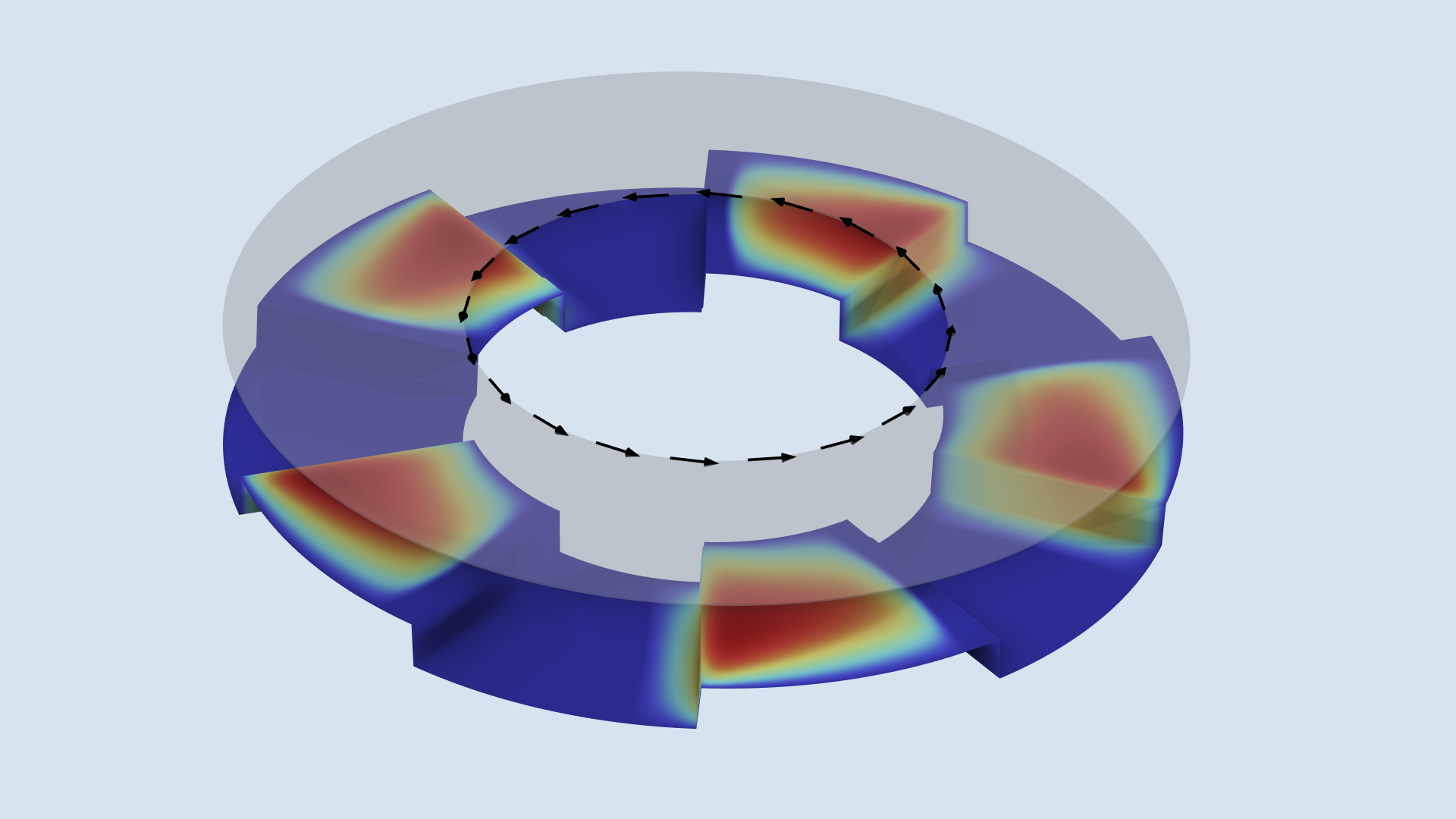
A step thrust bearing is sketched with the collar. The colors show the pressure. Note that the steps are not modeled in an explicit three-dimensional sense, so the plot does not represent the computational mesh.

The physics of the bearing is modeled with the Hydrodynamic Bearing interface in the COMSOL Multiphysics^® software. This feature does not consider the out-of-plane dimension explicitly. Instead, a planar geometry is used, and the thickness variation is accounted for directly in the equation, as shown in the image above.

The load carrying capacity depends on the pressure distribution, which in turn depends on the shape of the steps. Therefore, it makes sense to apply shape optimization to maximize the bearing capacity,

where \boldmath{f}_\text{c} is the distributed force acting on the collar, which consists of the Poiseuille, Couette, and normal pressure components. As mentioned previously, the model accounts for cavitation, but no attempt is made to limit the severity of the cavitation.

Shape Optimization

Shape optimization is performed by changing an existing shape using mesh deformations. There are a number of built-in functions for achieving this in the Shape Optimization interface, and in this particular case, a third-order Polynomial Shell feature is used where the out-of-plane deformation is disabled. This is used for one set of leading and trailing pad edges, and the mesh deformation is copied to the other pads using the Sector Symmetry feature.

The approach demonstrated here fixes the position of the points on the circular boundaries, but it’s possible to allow these points to slide along the circular boundaries. This, however, requires the use of equation-based modeling and separate Control Function features for the trailing and leading edges of the steps, and this complicates the setup. The increased design freedom only leads to marginally better performance, and therefore this blog post focuses on the simpler approach, but the alternative formulation is included in the Application Library of COMSOL^® version 6.1, and it can still be downloaded from the Application Gallery.

The result of the shape optimization is shown in the figure below. The result depends on the maximum deformation of the edges as well as the initial groove angle. The optimization yields a design that pushes the oil together along the middle before it’s forced over the pad.

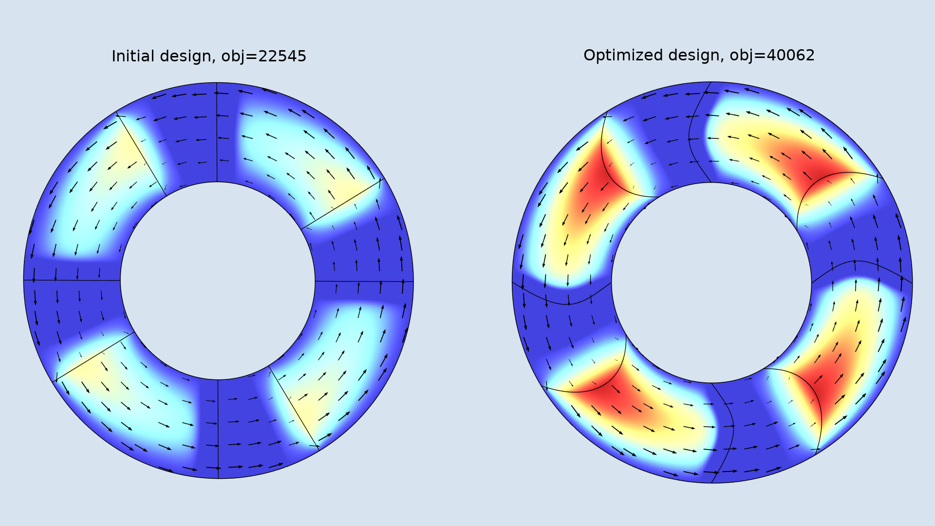
The initial design (left) is shown together with the optimized design (right). The mean fluid velocity is plotted with arrows and the colors show the pressure distribution.

It’s good practice to perform a verification by remeshing in the deformed configuration. The verification does not reveal any numerical problems, as can be seen in the Application Library version of this model.

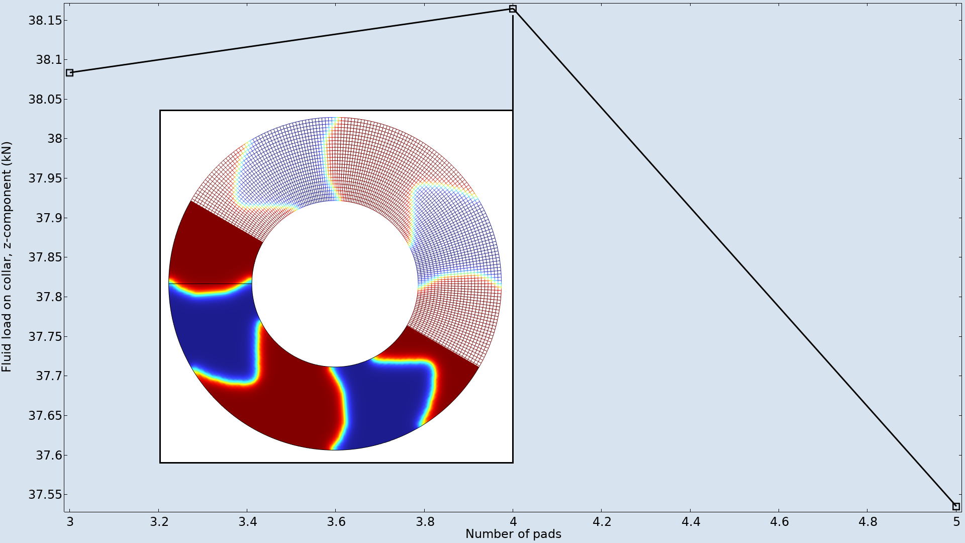
In this example, the maximum deformation and the groove angle are fixed to be independent of the number of pads. Because of this, the optimum number of pads is four, as illustrated below.

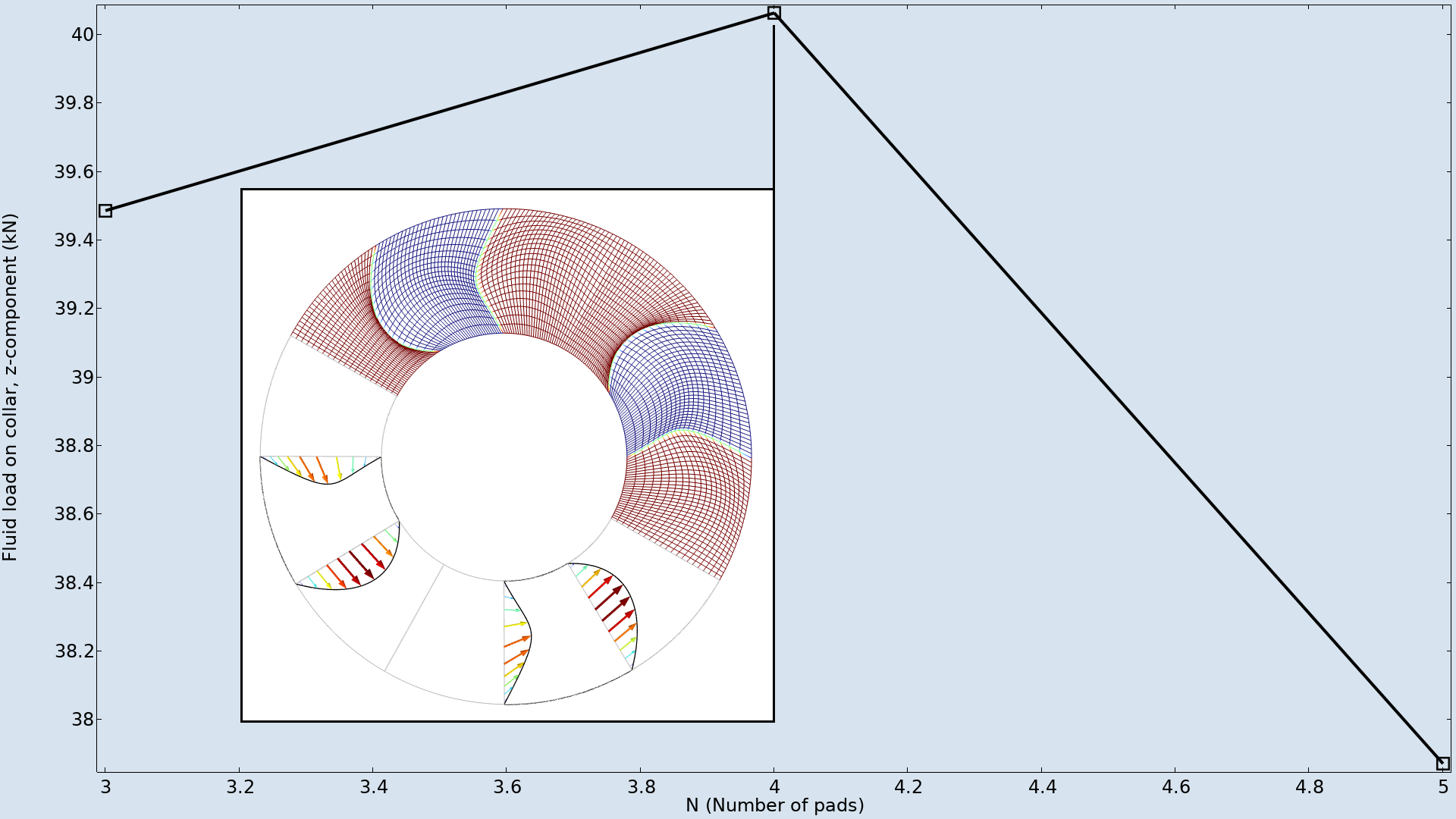
The shape optimization is performed for a different number of pads and the resulting objectives are graphed. The maximum occurs for four pads, and the inset shows how the mesh is deformed.

Shape optimization works the same regardless of the physics, and this makes it easy to set up. The mesh distortion that the shape optimization introduces is limited to avoid numerical problems, but the user is free to experiment with the balance between large design freedom with large performance improvement and small design freedom with robust optimization. In any case, the optimized design is very dependent on the initial geometry in the sense that the topology (and thus the number of steps) can only be an input to the optimization, not an output. Topology optimization can address this issue by introducing an implicit description of the geometry. The method can have its own disadvantages, but in this case it can be used without any significant complications.

Topology Optimization

Topology optimization works by introducing a design variable, \theta_c, for every computational element. This is confined to the closed interval between 0 and 1. It’s required that the variable is related to the physics such that:

1. Where the design variable is equal to 0, the governing equations corresponding to a groove is solved
2. Where the design variable is equal to 1, the governing equations corresponding to a pad is solved
3. Where the design variable is between 0 and 1, a governing equation combining the equations corresponding to a groove and pad is solved

The only difference between grooves and pads is the thickness of the oil film, h_f, so the abovementioned requirements are satisfied by letting this thickness depend on the design variable. For other topology optimization problems, the details of the third point require special attention, but in this case simple linear interpolation turns out to be sufficient:

where \theta_f is the field used in the physics, while \theta_c is the control variable field. In this case, one can set \theta_c = \theta_f, but convergence can be improved by introducing a filter that removes the small length scale in the control variable field. This also gives smoother results for results evaluation and verification. The filter can be expressed as a partial differential equation (Helmholtz filter),

where R_\mathrm{min} is the minimum length scale. (For more details on the Helmholtz filter and regularization for topology optimization, see our blog post “Performing Topology Optimization with the Density Method”.)

The optimization is free to set the design variable to intermediate values, and in this case one could interpret this as an intermediate oil film thickness, but oftentimes intermediate values don’t have a clear physical representation — or at least not a representation that is of practical relevance. This problem seems inherently well posed in the sense that the optimization automatically finds a solution without intermediate design variables, meaning that there is a clear distinction between the pads and the grooves.

It’s best to start topology optimization from a uniform value of the design variable. This results in a design with four pads, but one can also start from a nonuniform design to promote a different local optimum, as seen in the figure below.

The topology optimization is initialized with different nonuniform initial designs to promote certain topologies. The graph indicates that the optimal number of pads is four.

For these settings, there appears to be good agreement between the shape and topology optimization results.

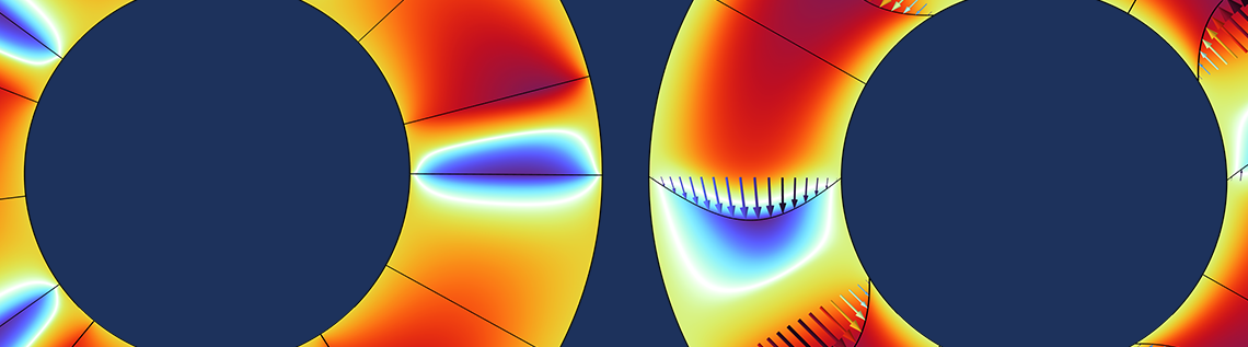
After performing topology optimization, it’s also good practice to perform a verification simulation, but where the verification for the shape optimization serves to check for numerical problems associated with deformed elements, the verification for topology optimization serves to check for problems associated with the implicit geometry representation. The verification for topology optimization thus uses an explicit geometry representation, and this produces a significantly better objective function, which indicates that there is a substantial cost to the implicit geometry description. Exploring this further, it’s found that it’s possible to get a significantly better objective with the topology optimization if one uses a finer mesh, as shown in the animation below, where the design has been initialized to promote a topology with 16 pads. The resulting design is qualitatively similar to the previous designs, and it’s similar to herringbone-grooved thrust bearings.

The topology optimization of a bearing initialized with 16 pads.

All of the optimizations consider a fixed rotation direction, and this is clearly visible in the optimized designs. The initial design is symmetric with respect to rotation axis, so it’s clear that performance can be gained by relaxing this constraint. Because of this, one would also expect smaller objectives if both rotation directions are considered in the optimization.

Conclusion

Here, we have discussed how shape and topology optimization can be used to design step thrust bearings. The setup of the physics and the optimization discussed here can be examined in these models and their associated documentation:

• Shape Optimization of a Step Thrust Bearing
• Topology Optimization of a Step Thrust Bearing

Further Learning

You can learn more about optimization by checking out the following resources:

• Read about these add-ons to the software that make the optimization of step thrust bearings (and more!) possible:
  • Rotordynamics Module
  • Optimization Module
• To learn more about the topology optimization of structural mechanics, check out these blog posts:
  • Performing Topology Optimization with the Density Method
  • Performing Topology Optimization with Milling Constraints