
Have you ever run a large parametric sweep overnight, only to discover the next morning that the parametric solver is still not finished? You may wish you could inspect the solutions for the parameters that are already computed while waiting for the last few parameters to converge. The remedy to this problem is to use a batch sweep, which automatically saves the parametric solutions that were already computed on a file that you can open for visualization and results evaluation purposes.
Editor’s note: This blog post was originally published on February 2, 2016. It has since been updated to reflect new features and functionality.
Batch Sweep: A Helpful Solution for Many Simulation Cases
In a previous blog post, we discussed the added value of task parallelism in batch sweeps. In this blog post, we will see how batch sweeps also fill another important purpose: retrieving solutions for a parametric sweep during the solution process. Using a batch sweep, you can sometimes retrieve partial solutions, even when the solver fails for some of the parameters. Batch sweeps are useful when the problem formulation is such that the solution for each parameter is independent of the solution of all other parameters.
There are many cases for which you may want to inspect the partial results during a solver sweep. For example:
- You are basing your sweep on a table of input data and it turns out that obtaining a solution for some of those tabulated values takes an unexpectedly long time, but you don’t know which values beforehand. You may still wish to inspect the solution for as many parameters as possible to determine if you should terminate the solution process or start analyzing the results before the entire sweep is complete.
- You are using a mathematical expression for a certain material property or boundary condition that turns out to give nonphysical results for some parameters.
- You wrote an external function in C or FORTRAN to define a complicated material, but you didn’t make it foolproof for all input data and it returns bad output data for certain parameter values.
- You are running a parametric sweep where one of the parameters is a geometric dimension, but you accidentally defined too wide of a range of dimensions. By the time you realize this, the solution has already been running for a long time and you don’t want to stop it.
If you use a batch sweep in any of these cases, each parameter can be solved for in a separate process that can be started and stopped independently. The results for the parameters that have already been solved for can be stored as an MPH-file for each parameter value and you can open and review any number of them during the solution process. In the example below, you will also see how to save probe results to a text file.
An Electrostatic Sensing Example
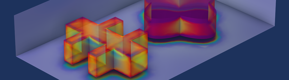
To demonstrate a batch sweep in action, we will use an example found in the Application Library of the COMSOL Multiphysics® core product: the Electric Sensor. This example model shows how to return an image of the interior of a box by applying a potential difference on the boundaries of the box. The result is a surface charge that depends on the permittivity of the medium inside the box and could be used to, for example, determine if there is an object in the box and even find information on the shape of the object. A similar technique, but with alternating currents, has applications in electrical impedance tomography for medical diagnosis.

The surface charge outside of the box.

The objects to be detected inside of the box.
The original model has the objects extruded to a thickness of 0.8 m. In this example, the extrusion distance was changed to 0.5 m.
Input Data for the Parametric Sweep
Let’s say that we have a set of ten sample objects, each having the same shape but made of different materials with different permittivity values. We would like to investigate the ability to detect the object and its shape, regardless of what it is made of. We store the permittivity values for the ten samples in an interpolation table, int1. We won’t actually use the table to interpolate anything, but merely as a convenient way of storing and calling the tabulated values. (Here, we could change the interpolation method from the default Linear to Nearest neighbor, but the results will be the same in this case.)
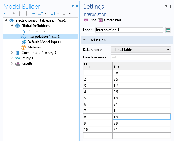
The table of permittivity values.
Let’s now index the sample set with a global parameter, sn (short for sample number).
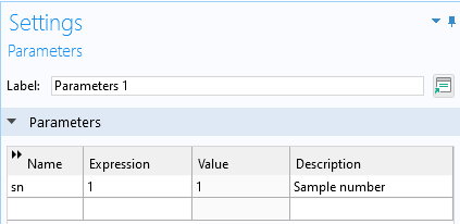
The sample number parameter, sn, as a global parameter.
The model has three materials defined under the Materials node. Material 3 represents the star-shaped object in the box and Material 2 represents the other object. Material 1 corresponds to the air surrounding the objects in the box. We change the permittivity of the star-shaped object with a suitable call to the interpolation table, int1, in the material property definition of Material 3. The syntax used is int1(sn). Note that we don’t need to worry about units, since permittivity is unitless.

The permittivity of the star-shaped object is taken from a table indexed by the parameter sn.
Probing the Surface Charge
To monitor the surface charge above the star-shaped object, we define a Boundary Point Probe located at the top surface at the location x = 1.5, y = 1.5, z = 1.0. To define this quickly, we can simply click on the surface at an approximate location above the object and then adjust the coordinate values manually in the Settings window.

A Boundary Point Probe above the object of interest.
For the Point Probe Expression, we choose the magnitude (norm) of the surface charge with the variable name es.nD and unit nC/m^2.
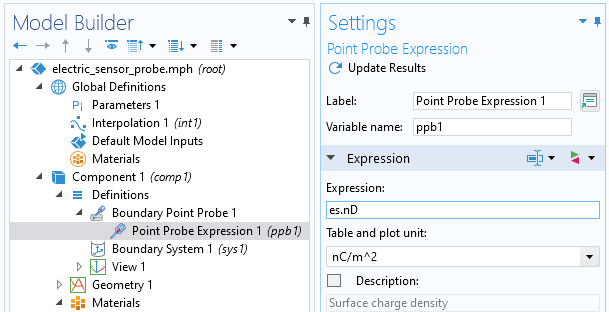
The Point Probe Expression for surface charge in units of nC/m^2.
We will later write the output of this probe to a text file. To prepare for that step, click on Update Results. This generates a Derived Values and Table item.
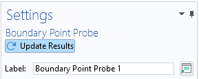
The Update Results button for the probe.
Setting Up the Batch Sweep in COMSOL Multiphysics®
The Batch Sweep option is not visible by default. To enable it, select Show More Options from the Model Builder toolbar. In the Show More Options dialog box, select Study>Batch and Cluster.

The Advanced Study Options, activated in the Show More Options menu of the Model Builder.
If we right-click on the Study node, we can select Batch Sweep in the list (selecting Batch instead of Batch Sweep is used for single runs).
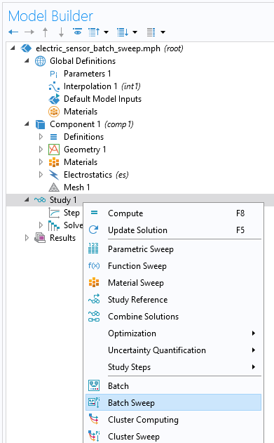
Selecting Batch Sweep from the Study menu.
A batch sweep is similar to a parametric sweep with regards to how the sweep range is defined. Here, we sweep the parameter sn from one to ten in integer steps.
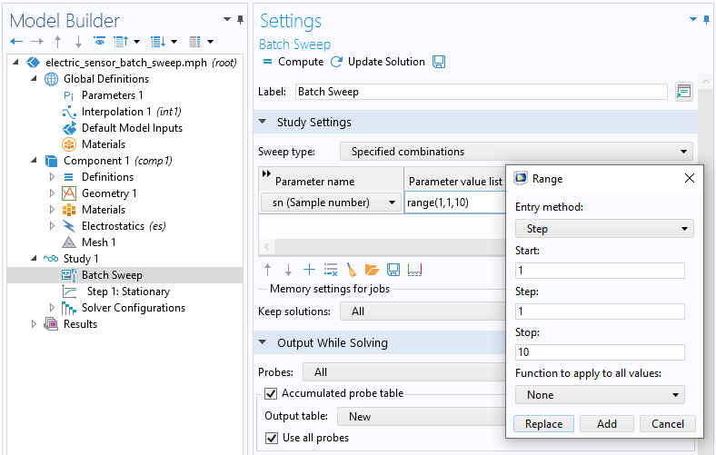
The parameter range for the batch sweep.
The settings for controlling what should happen to the results are collected in the Batch Settings section of the Settings window, found in the Batch Sweep model tree node.
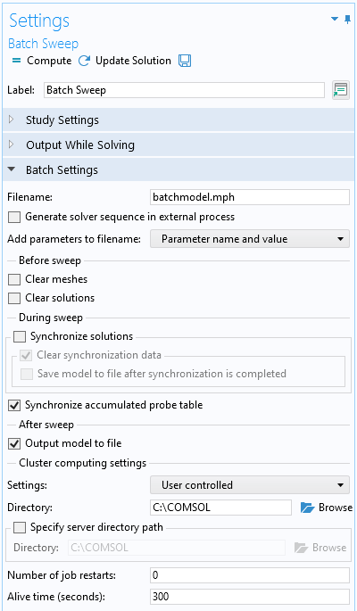
The settings for controlling a batch sweep.
The default filename is batchmodel.mph. This name is used to automatically create a sequence of MPH-files corresponding to each individual parameter in the sweep. We could change this name, but for the purposes of our example, we’ll keep it as is. The resulting names of the MPH-files are batchmodel_sn_1.mph, batchmodel_sn_2.mph, …, and batchmodel_sn_10.mph. We see below how each of these files is a fully fledged model that can be opened and postprocessed separately.
The Before sweep section has two options: Clear meshes and Clear solutions. We clear these check boxes, since they are only really important when we perform a remote computation on a cluster or cloud and wish to minimize the size of the file transferred over the network (only available with a floating network license).
The During sweep section has two options: Synchronize solutions and Synchronize accumulated probe table. Synchronize solutions takes the results from all of the stored files and collects it in the “main” MPH-file from which we are starting the simulation. The net result is very much like that of running a parametric sweep. In our example, we clear this check box since we assume that we are only interested in inspecting the individual results. Furthermore, if you have a large sweep, collecting all of the results may consume a lot of time, RAM, and disk space. We keep Synchronize accumulated probe table selected. The accumulated probe table represents the output from the probe, and collecting this information is very light compared to the full solution information.
Under After sweep, we select the Output model to file check box. This ensures that the MPH-files that are automatically saved contain the solution (for each parameter), at the cost of additional disk space.
In the next section, change the Cluster computing setting to User controlled. Then, change the Directory to C:\COMSOL. This is the location where all of the batch files are stored.
You can use the Specify server directory path option if you have a floating network license and wish to perform this computation using an installation at a remote location. Here, we only cover features that are available in all types of COMSOL licenses, including single user licenses.
Save the Probe Data on File
In order to save the probe data to a file, we cannot use the regular probe table. Instead, we need to use a special kind of probe table called the Accumulated Probe table. The first step is to manually add a probe table by right-clicking on the Table node under Results. Change the name of this table to Saved Probe Table. We will soon let the batch sweep machinery write the data for the Accumulated Probe table here. An Accumulated Probe table is used when we have asynchronously generated data that should be put in a certain order in a table. Remember that in general, we don’t know in what order the solutions corresponding to the different parameters will be ready. The Accumulated Probe table will take care of this for us.
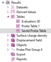
Manually adding a Saved Probe table.
In the settings for the Saved Probe table, we change the Store table setting to In model and on file. In this example, we are saving the probe results to C:\COMSOL\results.txt. If you have a very large sweep, you may need to increase the value for Maximum number of rows. (This is typically needed for large sweeps or transient solutions.)
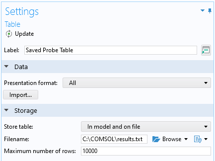
The Saved Probe Table settings.
In the settings for Batch Sweep, in the section Output While Solving, change the Output table to Saved Probe Table. This will now be our Accumulated Probe table.
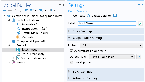
Using the Saved Probe table as an Accumulated probe table.
Running the Batch Sweep
We can now click on or select Compute to start the batch sweep. While solving, the External Process window is visible in the information window area below the Graphics window.

The External Process window.
In the External Process window, we get an overview of the running batch processes and their status. In our example, there are ten such processes corresponding to each parameter in the sweep.
At this stage, large parts of the user interface are noninteractive, but we can click on Detach job to the left of the progress bar to regain control of the user interface.
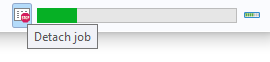
The Detach job option.
While using Detach job, we don’t get live updates of the process status. However, we can now perform operations on the individual processes.

The detached External Process window.
We can now stop all processes or click on a row and stop that particular process. We can even click on a process in the table with the status Done and open it up in a separate COMSOL Desktop® window. There, we can perform any kind of visualization or postprocessing task that we would normally perform on a model.
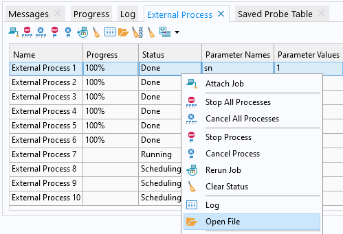
Clicking on Open File for a completed external process opens a new window in the COMSOL Desktop® with the results.
To get back to the live update of the process status, click on Attach Job in the upper left corner of the External Process window.
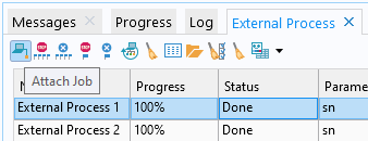
Attaching the External Process window.
The Probe Results File
We can use a text editor to open the file results.txt, which contains the probe output.
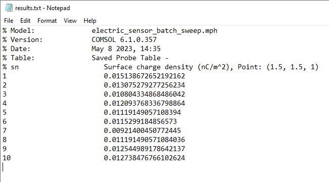
The text file results.txt, containing the boundary point probe results.
This file will also be available for inspection during the solution process and can serve as a very quick way of peeking at the results before all of the parameters have converged. This is true not only for batch sweeps, but also for tables saved to a file for regular parametric sweeps.
Other Factors to Consider when Using Batch Sweep
Performance
For a sweep where each computation is quick and doesn’t require much memory, such as this example, the computation time using a batch sweep is longer than if you used a regular parametric sweep. The overhead comes from the fact that for each parameter, a separate COMSOL Multiphysics® process is started. For sweeps where the computation for each parameter is more demanding, this time is relatively smaller and less of a concern.
Handling of Crashes for Certain Parameters
Let’s say that we, instead of the interpolation table, called a user-defined external C function. Furthermore, let’s say that we made a programming error in the C code that resulted in a segmentation fault for one or a few of the parameters for which we are sweeping. In this case, we can still browse to the C:\COMSOL directory (or whatever directory you choose to store your MPH-files) and open those files for visualization and postprocessing, or even further computations.
An easy way to emulate this in the above example is to set one of the permittivity values to zero and start the batch job. A zero permittivity means that we are feeding the solver with an ill-defined (even singular) equation (similar to 0 = 1) and you will get an error message indicating that the solver couldn’t find a solution corresponding to that erroneous parameter. Again, you can still open and postprocess the saved MPH-files. If you correct the table by changing the entry to a nonzero entry, you can run the batch job again without getting error messages. Note that while the error exists, you cannot attach the External Process window without getting an error. The Accumulated Probe table is still updated for the other parameters when you attach the window. As soon as you correct the error and run, you can again access the External Process window by attaching it.
Managing Multicore Processing
If you have a multicore machine, which is very likely these days, then you can change the Batch settings that control the number of simultaneous processes that are allowed to run in the batch sweep and also how many cores each of them is allowed to use. If you have a six-core machine, then you could, for example, change the Number of simultaneous jobs to three and the Number of cores to two. This allows three parameters to be solved in parallel, where each solver process gets access to two cores and, for this example, cuts the simulation time in half.
For simulations where each parameter represents a small computational problem, you can increase the number of simultaneous jobs to as many cores as you have on your computer. For larger problems, you should keep this setting to one simultaneous job to fully utilize the multicore processing power of the solvers.
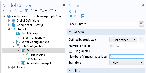
Batch settings for simultaneous jobs and the number of cores.
Note that you can also control the Number of simultaneous jobs from the Batch Sweep node, under the section Study Extensions. In this case, the number of cores will be automatically computed from the number of physical cores divided by the number of simultaneous jobs. (For this to be automatic, you must not select the Number of cores check box under Batch settings. The grayed-out Number 1 will not be used.)
Batch Sweeps and the Application Builder
With the Application Builder, you can use a Batch Sweep node in a model that is used to build an app. In this case, the app will serve as the “driver” of the batch sweep and you cannot see the information in the External Process window. The saved MPH-files will serve the same purpose, as if you didn’t have any user interface for the app. The files can be opened for conventional model postprocessing when the run is finished. In order to get more flexibility when creating an app that uses Batch Sweep, use a method that includes the built-in methods for Batch Sweep, as listed in the Programming Reference Manual. (Note that the Record Code tool is of limited use here, since the generation of the recorded code will conflict with the live run batch commands.)
Batch Sweeps Versus Cluster Sweeps
The Batch Sweep feature is available for all COMSOL Multiphysics® license types. If you have a floating network license, then you have access to an additional feature called Cluster Sweep. These two features are similar, but the Cluster Sweep option has additional settings for remote computations and cluster configurations. The Cluster Sweep feature lets you distribute a large sweep on a (potentially large) cluster. The performance benefit of doing so can be very high, since independent sweeps (also known as embarrassingly parallel computations) typically scale very well. If you master the batch sweep, then the step toward running a cluster sweep isn’t that big.
Next Steps
Want to explore the models discussed in this blog post for yourself? Download them via the Application Gallery:
Further Learning
Learn more about batch sweeps and cluster sweeps by checking out these articles on the COMSOL Blog:


Comments (15)
Alexey Trukhin
February 3, 2016Dear Bjorn,
Great a blog! Finally, it is clarified what is the difference between the ‘Parametric sweep’ and the ‘Batch sweep’. As for me, the documentation provided with the COMSOL is quite vague on the topic.
Kind regards,
Alexey
Bjorn Sjodin
February 3, 2016Hi Alexey,
I’m glad you liked the posting!
Best regards,
Bjorn
James Freels
February 8, 2016Hello Bjorn,
Thank you for publishing this great blog article. This information will prove very useful for us going forward.
Bjorn Sjodin
February 8, 2016Hi James,
You’re welcome!
Cheers!
Bjorn
Pablo Rodriguez
February 18, 2016Hi Björn,
Thanks for clarifying the usage of batch sweeps. There are a few things which are still not clear though. How do you indicate the data to collect in the accumulated probe table? Before performing the calculation there are no values to insert and thus no obvious way to fill in the column headers. Perhaps I am missing something obvious but I am unable to manually insert the column headers directly under the table settings
For radio frequency studies, the non-parameterized study uses a frequency sweep (Study -> “Step 1: Frequency Domain”). If I want to collect multifrequency data for different parameter combinations using a batch sweep, do I have to move the frequency sweep into the batch sweep and set the Frequency Domain value to a parameter? Put another way, instead of generating n frequency points for m batch sweep parameters, do I have to generate unique points for n*m batch sweep parameters? If not, how can I accumulate multi-point data (graphs) for each batch sweep parameter combination?
It would be helpful if you could include an example of launching a batch-sweep from the command-line. Using e.g. comsol batch -inputfile foo.mph -outputfile foo_out.mph -study std1 doesn’t seem to work and the different parameter combination output files were not generated. I suppose that one must append “-job batsw” but I haven’t had time to test it yet. Can “-pname” and “-plist” be used to configure non-swept parameters?
The command-line usage will vastly increase productivity if it works as expected yet documentation is sparse and the forum threads are often lacking in clear and concise information.
Thanks in advance for any further information and help that you can provide.
Regards,
Pablo
Bjorn Sjodin
March 22, 2016Hi Pablo,
I’m glad you found the blog post interesting. I will try to address your questions.
The accumulated probe table is an accumulation of all probes in the model so there is no need for you to setup the table. It is automatically created from the probes you are using.
(Assuming I understand the question correctly) You can perform a batch sweep for m parameter values and perform the frequency study for the n frequency variation you are interested in in the Frequency Domain step. This will create n*m data. Similar to if you had a Parametric Sweep instead of a Batch Sweep.
There is no command line support for running Batch Sweeps. They have to be initiated from the GUI.
I hope this helps.
Bjorn
Ruslan Prozorov
November 19, 2017What if I do not use probes at all, but instead calculate several parameters in “derived values”. Some refer to global variable which themselves are integrals over domain etc? What if I sweep not one, but more parameters in ALL combinations (think of a 2D matrix of values)? It would help if, instead of very specific EM model you could illustrate, for example, how to calculate the volume and surface area of an ellipsoid when I vary the values of a,b and c – semiaxes. Each, a,b and c varies from 1 to 10 and I need ALL values to output into a single table. (There will be 1000 of them). The volume is calculated as a volume integration and surface area as a surface integral. So, the table will contain 5 columns: a,b,c,vol,surface.
Bjorn Sjodin
November 21, 2017Hi Ruslan,
Yes, this would be a natural extension of a one parameter sweep. However, from a user interface point of view it is not much different. For a general example of a multiparameter sweep (two parameters) see for example:
https://www.comsol.com/video/performing-parametric-sweep-study-comsol-multiphysics
Best regards,
Bjorn
Buccma Accumulator
June 28, 2023Your article is very nice & informative, thanks for the sharing with us.
Jim Freels
June 28, 2023Dear Bjorn,
Thank you very much for a very helpful article. One question: Is it possible to run COMSOL in batch mode by adding batch switch on the command line, and utilize the batch sweep ? Obviously the interactive features would not be there, but the ability to create several output files from different parameters would be helpful in a batch mode.
Bjorn Sjodin
June 29, 2023 COMSOL EmployeeHi Jim,
You are welcome! Yes, there are a few ways to do this. If you have an MPH-file with a regular study and no Batch sweep node in the study, then you can get a similar behavior by issuing a command like:
comsol batch -inputfile electric_sensor_plain.mph -outputfile electric_sensor_plain_solved.mph -batchlog b.log -pname sn -plist 1,2,3,4,5,6,7,8,9,10
This will generate a series of files: electric_sensor_plain_solved_sn_1.mph, electric_sensor_plain_solved_sn_2.mph, electric_sensor_plain_solved_sn_3.mph, etc. with separate solutions for the different values of the global parameter sn
If you would like all the solutions to be synchronized into one final MPH-file then you would need to use the user interface and add a Batch node. After this you could issue a command such as:
comsol batch -mode desktop -inputfile electric_sensor_batch_sweep.mph -outputfile solved_batch.mph -batchlog b.log
where -mode desktop tells COMSOL to use the batch settings of the user interface.
The syntax I used here is for Linux but it is similar for Windows (see the section The COMSOL Commands in the COMSOL Reference Manual).
I hope this helps.
Bjorn
Jim Freels
July 2, 2023Bjorn, Thank you. I was unaware of everything you mentioned here. Thanks again, and Happy 4th of July !
Bjorn Sjodin
July 3, 2023 COMSOL EmployeeHi Jim,
You’re welcome and Happy 4th of July!
Bjorn
trennie grenn
July 24, 2023The use of batch sweeps, as you mentioned, can indeed be helpful in such scenarios. By automatically saving the parametric solutions that were already computed, you can analyze the results and evaluate the progress while waiting for the remaining parameters to converge. The continuous development and updates to simulation software, including new features and functionalities, contribute to improving the efficiency and effectiveness of parametric sweeps, making them an essential tool in engineering and research.
Bjørn Vik
August 3, 2023Hi Björn,
It would be interesting to see a a similar post where you use model manager in combination with batch sweep.
Cheers
Bjørn