

Previously, you saw how to compute stiffness of linear elastic structures in 0D and 1D. Today, we will expand on that and show you how to model this in 2D and 3D. We will also show you an alternate method to compute stiffness.
Including the Poisson Effect and Shear Modulus
In Part 1, we showed you how the shear effect introduced by the Timoshenko Theory affected the stiffness. Now, let’s try to incorporate another realistic effect in this model such that when the beam is pulled along its length and elongates, its cross-sectional area will be reduced. This is known as the Poisson effect. The ratio between the transverse and axial strains is denoted by the material property known as Poisson’s ratio (\nu ).
In general, the Poisson effect is incorporated in the physical description of a linear elastic deformation through the material’s stiffness matrix, [C], which relates the stresses, {σ}, and strains, {ε}. Hooke’s law is modified to account for both axial and shear components along different directions. In its generalized form, it can be written like this:
Note that the material’s stiffness matrix, [C], is a material property, as opposed to the structural (or device) stiffness (k) that we had introduced earlier.
For isotropic linear elastic materials, the components of the material’s stiffness matrix, [C], can be evaluated using only the material’s Young’s modulus and Poisson’s ratio, as the shear modulus is a function of these two parameters. For orthotropic materials, we would need to specify unique values for the Young’s modulus, Poisson’s ratio, and shear modulus. For a general anisotropic linear elastic material, the stiffness matrix could consist of up to 21 independent material parameters that take care of both Poisson’s effect and the shear effect along different directions. Although our example model uses an isotropic material, the ideas discussed in this blog entry hold true for orthotropic and anisotropic materials as well.
Now, let us find out how these effects can be incorporated in our beam model in different space dimensions. We will use a Poisson’s ratio of 0.3 (~ shear modulus of 77 GPa) for all our computations.
2D Model
When modeling the beam in 2D, we could choose between a plane strain or a plane stress assumption. In COMSOL Multiphysics, you can model the 2D plane stress and plane strain cases by selecting a 2D space dimension and choosing the Solid Mechanics interface. The interface provides a drop-down menu to switch between “plane stress” and “plane strain” conditions.
Plane Strain Option
The “plane strain” option is suitable when there are only in-plane axial, shear, and bending forces acting on a structure, producing in-plane strains. The out-of-plane strain components are assumed to be zero. A typical example would involve a structure that is fully constrained in the out-of-plane direction. Hence, this is not an appropriate choice for modeling our beam example. In the “plane strain” formulation, the COMSOL software solves for the in-plane displacements, u and v.
Plane Stress Option
The “plane stress” option is suitable when there are only in-plane axial, shear, and bending forces acting on a structure, producing in-plane stresses. The out-of-plane stress components are assumed to be zero. In the “plane stress” formulation, COMSOL Multiphysics solves for the in-plane displacements, u and v, as well as the out-of-plane strain, (wZ ). For an anisotropic material, it additionally solves for the out-of-plane displacement gradients, uZ and vZ . That’s why, in COMSOL Multiphysics, you can use the 2D “plane stress” modeling interface even for anisotropic materials, as long as the boundary conditions support the plane stress assumption. There are several combinations of boundary conditions that would support this assumption. One such example is a beam subjected to a roller boundary condition at one end and free at the other.
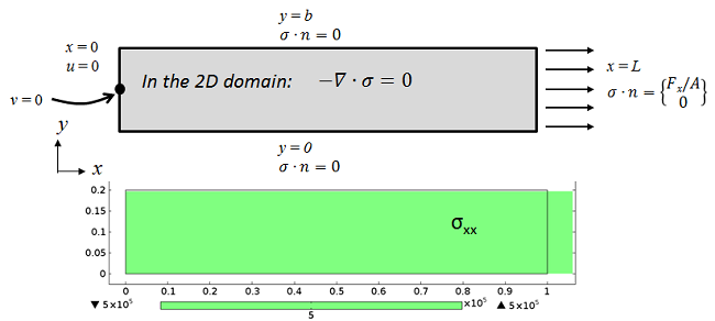
Boundary conditions showing “ideal” plane stress conditions on the beam subjected to axial load. The roller boundary on the left helps in obtaining a constant value of the axial stress σxx. A geometric point at the center of the roller boundary has been used to constrain the y-displacement (v) to prevent in-plane translation.
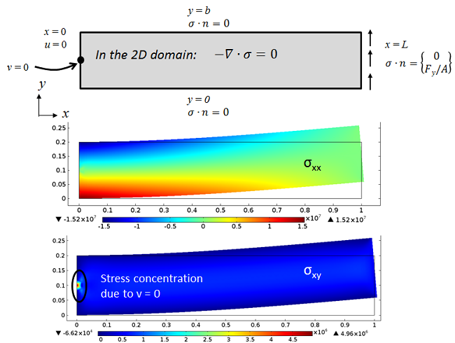
The same “ideal” plane stress beam subjected to transverse load. The bending stress, σxx, shows a smooth expected variation, but the shear stress, σxy, is singular around the point where v is constrained.
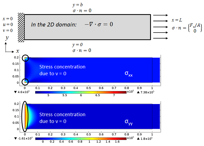
Boundary conditions showing fixed-free beam subjected to axial load modeled using plane stress assumptions. The axial stress, σxx, is singular at the corners as a result of constraining the transverse displacement. Due to the same constraint, we also receive a nonzero σyy because of the inhibited contraction in the vertical direction.
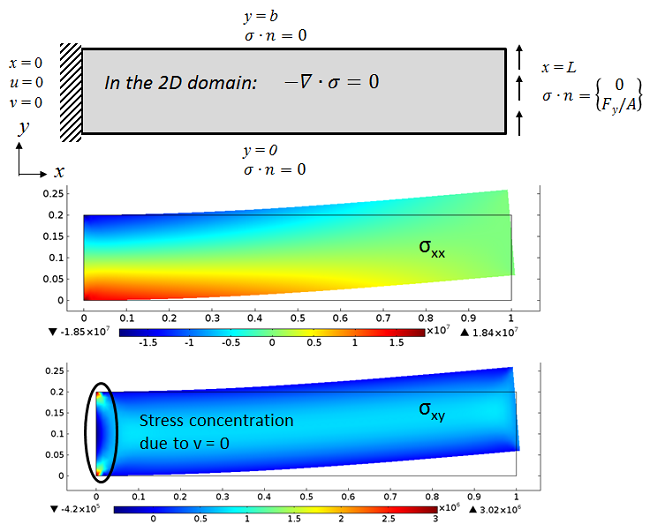
The same fixed-free beam subjected to a transverse load. The bending stress, σxx, shows a smooth expected variation, but its maximum value is slightly higher than what we get from the “ideal” beam. This is because of the additional stiffness arising from constraining the transverse displacement. As a result of the same constraint, we also receive singular values of σxy above and below the mid-plane of the beam.
The pictures above show that our fixed-free beam example can only be “approximately” modeled using the 2D plane stress assumption. Note that in the 2D model, the local y-axis can correspond to either the y-axis or the z-axis of a Cartesian coordinate system representing a 3D space, depending on whether we are representing the xy-plane or xz-plane in 2D.
Similarly, the transverse displacement, v, in the 2D model could represent either of the transverse displacements v or w of the 3D model, depending on whether we are representing the xy– or xz-plane. We can use this information to compute both the bending stiffness kyy and kzz by solving the model twice: once with a height of b (0.2 m) and then with a height of t (0.1 m).
Let’s look at the effect of these ideal and real boundary conditions on the stiffness computed by the 2D model:
| kxx [N/m] | kyy [N/m] | kzz [N/m] | |
|---|---|---|---|
| Roller-Free | 4×10⁹ | 3.86×10⁷ | 9.91×10⁶ |
| Fixed-Free | 4.01×10⁹ | 3.89×10⁷ | 9.94×10⁶ |
These values show that a realistic fixed constraint, as opposed to an idealized roller constraint, would lead to slightly higher values of stiffness due to localized stiffening effects near the fixed end. Note that for both these cases, the bending stiffness is lower than that of the Euler-Bernoulli Beam due to additional shear flexibility (i.e. accounting for shear deformation) in 2D models. Hence, these results are closer to the 1D Timoshenko beam models. (You can find the results from the 1D simulation in our previous blog post.)
3D Model
The 2D modeling approach is useful as long as there are no out-of-plane forces acting on the structure and the in-plane forces do not vary along the out-of-plane direction. For more general loading conditions and constraints on the structure, a 3D model could provide more accurate information, but be more computationally taxing. For a true 3D model, you would need to choose a 3D space dimension and the Solid Mechanics interface.
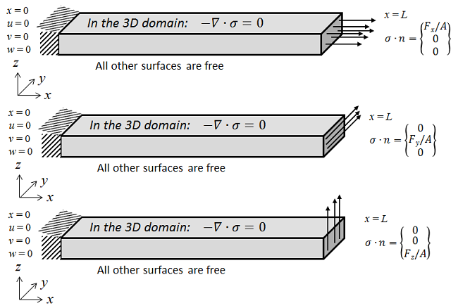
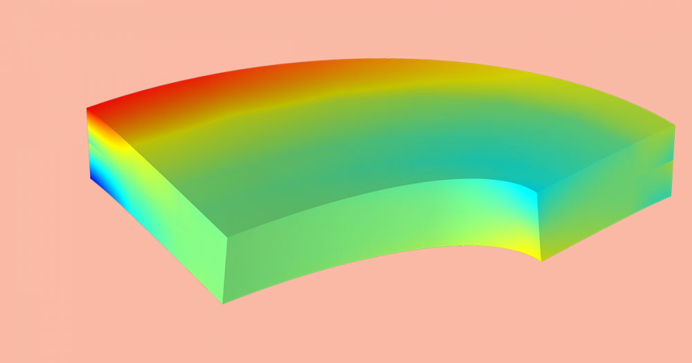
A 3D representation of the fixed-free beam subjected to axial and transverse loads. Solving the model for these three load cases allows us to evaluate the axial and bending stiffness.
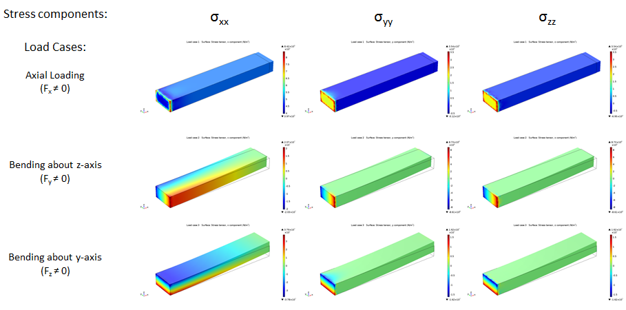
Summary of axial stresses for the three load cases. Note the stress concentration at the fixed end that arises from a combination of the fixed constraint boundary condition and coupling of strains along different directions via the Poisson effect.
Next, let’s look at the axial and bending stiffness computed by the 3D model. We will compute the stiffness for two cases: first by setting Poisson’s ratio to 0.3, then by setting it to 0. This will allow us to compare the 3D results with the 1D beam theory results.
| Poisson’s ratio | kxx [N/m] | kyy [N/m] | kzz [N/m] |
|---|---|---|---|
| ν = 0 | 4×10⁹ | 3.91×10⁷ | 9.94×10⁶ |
| ν = 0.3 | 4.02×10⁹ | 3.92×10⁷ | 1.006×10⁷ |
Note that for a Poisson’s ratio of 0, the results match perfectly with those when using the 1D Timoshenko beam theory. For a Poisson’s ratio of 0.3, the Timoshenko theory predicts a lower bending stiffness as a result of accounting for the shear flexibility. However, the 3D model predicts a slightly higher axial and bending stiffness as a result of the fixed constraint boundary condition, which produces an additional stiffening effect that offsets the shear flexibility, especially when bending in the least shear-flexible direction.
The realistic effect we have seen here could unfortunately have been neglected, had we not modeled the structure in 3D.
Stiffness or Compliance?
Now we’ll revisit the method that we have used so far to compute the stiffness.
We fixed one end of the beam and applied a force at the other. We varied one component of the force vector at a time by making it nonzero (and left the other force components as zero) and evaluated the resulting average tip displacement of the beam. Under these conditions, the force vector (F) and displacement vector (u) should strictly be correlated using a compliance matrix, [s], such that \bold{u}=[s]\bold{F}.
The same equation can be written in a matrix formulation:
Here, the compliance component, sij, denotes the linearized compliance relating the amount of incremental displacement you get along the i th direction (where i can be x, y, z) when we apply an incremental force along the j th direction (where j can be x, y, z). We will call this approach as the force-controlled method.
Based on our previous definition of stiffness, we can now define a general stiffness matrix such that \bold{F}=[k]\bold{u}.
We can represent that in a matrix formulation, too:
In the stiffness matrix, the diagonal terms correspond to axial and bending stiffness and the off-diagonal terms denote any stiffness due to extension-bending coupling. In absence of such extension-bending coupling (as in our case), we receive a diagonal compliance matrix. Therefore, we could say that kxx = 1/sxx, kyy = 1/syy, and kzz = 1/szz. This is what we have used so far.
Note that the input to the second matrix formulation is equal to the different components of displacement, while the output of interest is equal to the components of the reaction force that is “felt” at the boundary with the prescribed displacement. So, in order to find the different components of the stiffness matrix, we need to vary one component of the displacement vector at a time, by making it nonzero (and setting the other displacement components to zero), and evaluate the resulting reaction force.
The so-called “free end”, where we were applying the axial and transverse loads, is not free anymore. Based on this, we can now say that the stiffness component, kij, denotes the linearized stiffness relating the amount of incremental reaction force that you get along the i th direction (where i can be x, y, z) when we apply an incremental displacement along the j th direction (where j can be x, y, z). We will call this approach the displacement-controlled method.
Can There Be any Other Stiffness?
So far, we have limited our discussion to axial and bending stiffness that were obtained using forces and displacements. However, in reality, at any point in space, a structure can have six degrees of freedom, three of which correspond to translations while the other three correspond to rotations. Similarly, instead of only applying a force on a boundary in one of the directions parallel to x, y, or z, it is also possible to apply moments about these three axes.
For a cantilevered beam like ours, a moment about the x-axis would produce torsion, whereas moments about y– and z-axes would produce bending. All this information can be represented using the following matrix formulation:
This shows that we can have a general six-by-six stiffness matrix that could accommodate several types of stiffness terms such as axial, shear, bending, and torsion, as well as coupled terms between these modes .
Computing Stiffness in COMSOL Multiphysics: Alternate Method
With the new information in hand, let’s revisit our beam model:
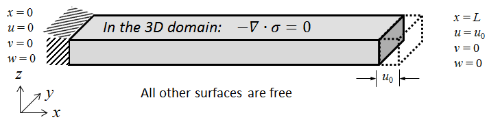
The beam model defined in 3D showing how we can prescribe the displacement at the tip of the beam.
In order to implement the displacement-controlled method in COMSOL Multiphysics, we would need to do the following:
- Find a way to prescribe the displacements on the boundary of the beam at x = L
- Find the reaction forces on the boundary of the beam at x = L
Prescribing the Displacement
If we use the Beam theory models (for 1D analysis), they would allow us to work explicitly with all six degrees of freedom (displacements and rotations). So, we could replace the Point Load with a Prescribed Displacement/Rotation, where we can set the displacement to some nonzero value (say, 1 mm) and at the same time not impose any constraint on the rotation at the tip of the beam.
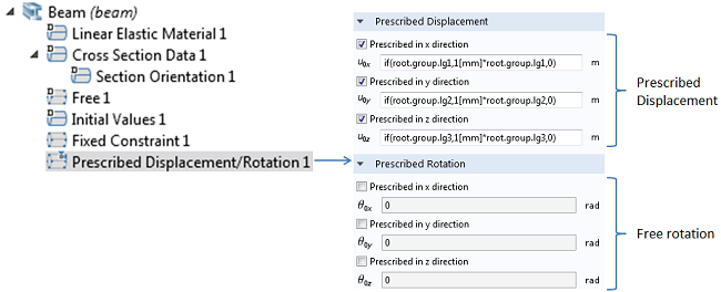
The Prescribed Displacement/Rotation feature applied at the tip of a 1D beam. A free rotation is allowed.
As shown in the previous blog post, we can use the if() operator and the names (such as root.group.lg1) associated with the Load Groups, such that only one component of the displacement vector can be made nonzero at a time when you are solving the same model for several load cases.
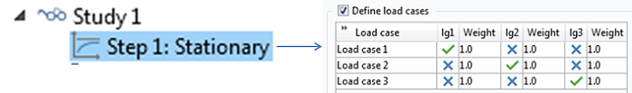
A snapshot showing how you can set up three load cases and solve the model with only one active load group at a time.
When using the Solid Mechanics model (in 2D and 3D), we can only specify or compute the three translational degrees of freedom (displacements), which are in turn used to compute the rotations. This also means that when we set up a displacement-controlled stiffness computation, the Beam theory easily allows us to either constrain the rotation or allow free rotation at a point.
In the Solid Mechanics model, on the other hand, it is not possible to freely prescribe or constrain the rotation everywhere on that surface by decoupling the rotation from the displacement. That is because we are dealing with spatial variation in displacement on a boundary. This means that if we simply assign a set of prescribed transverse displacements (say u = 0, v = 1 mm, and w = 0), it will fully constrain the rotation (i.e. Φx = Φy = Φz = 0), thereby increasing the effective bending stiffness of the beam. This is where the COMSOL software’s Rigid Connector boundary condition comes in and helps us overcome that problem in 2D and 3D solid models.
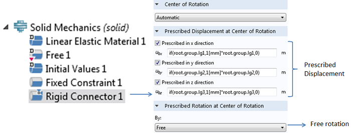
The Rigid Connector feature applied at the boundary of a 3D beam. Free rotation is allowed at the centroid of the boundary.
In our model, we could use similar expressions as shown earlier to prescribe the displacements in the Rigid Connector boundary condition to vary each of the displacement components, one at a time, using Load Groups and Load Cases. The Rigid Connector will introduce the same kind of local stiffening and stress disturbances as the Fixed constraint at the other end of the beam.
Computing the Reaction Force and Stiffness
The reaction force can be computed by setting up an Integration Coupling Operator that can be used to sum up the reaction force over all the nodes on a boundary. COMSOL Multiphysics provides predefined variables such as solid.RFx, solid.RFy, and solid.RFz that allow you to access the reaction force. The stiffness can then be computed as the ratio of the total reaction force and the value of the prescribed displacement at the tip of the beam. Alternatively, using an average of the displacement at the tip of the beam can be useful if the beam has an extension-bending coupling. In that case, the average displacement in a direction perpendicular to the load application will not be zero.
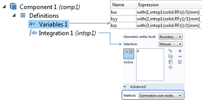
Screenshot of the Integration Coupling Operator and variables defined to compute the stiffness.
Summary of Axial and Bending Stiffness
Finally, here’s a summary of all axial and transverse stiffness values that we have computed in different space dimensions by either neglecting or including the Poisson and shear effects. The stiffness values obtained from both the force-controlled and the displacement-controlled methods agree closely with each other, thereby providing a consistency check:
| Space dimension (Poisson’s ratio) | kxx [N/m] | kyy [N/m] | kzz [N/m] |
|---|---|---|---|
| 1D Euler-Bernoulli | 4×10⁹ | 4×10⁷ | 1×10⁷ |
| 1D Timoshenko (ν = 0) |
4×10⁹ | 3.91×10⁷ | 9.94×10⁶ |
| 1D Timoshenko (ν = 0.3) |
4×10⁹ | 3.88×10⁷ | 9.92×10⁶ |
| 2D Plane Stress (ν = 0) |
4×10⁹ | 3.91×10⁷ | 9.94×10⁶ |
| 2D Plane Stress (ν = 0.3) |
4.02×10⁹ | 3.89×10⁷ | 9.94×10⁶ |
| 3D (ν = 0) |
4×10⁹ | 3.91×10⁷ | 9.94×10⁶ |
| 3D (ν = 0.3) |
4.04×10⁹ | 3.92×10⁷ | 1.01×10⁷ |
Conclusion
We have now explored the concept of axial and bending stiffness of structures in more detail. We started with a conventional definition of stiffness, which is suitable for 0D models, and expanded it to fit assumptions and theories available to model structures in 1D, 2D, and 3D that involve multi-axial loading. We saw that the stiffness of a structure can rarely be captured by a single-valued number.
Structural stiffness could be affected by several other factors that we have not explored here. Some of these include:
- Geometric nonlinearity:
- What happens when the stiffness becomes a function of the magnitude of force or displacement?
- Material nonlinearity:
- How do we define the stiffness of materials, such as metals above yield strength or rubber that do not follow Hooke’s law?
- Multiphysics:
- How do we define stiffness when a non-mechanical load, such as thermal or fluid, produces structural displacement?
Next Steps
- Read the previous blog post in this series: Computing Stiffness of Linear Elastic Structures: Part 1
- If you have any questions about computing stiffness using COMSOL Multiphysics, please contact us

Comments (5)
Lingling Tang
April 5, 2014Thanks for your sharing, Datta. This blog and the former one is instructive.
Supratik Datta
April 7, 2014Hi Lingling, I am glad you found this post helpful. Thanks.
haider alrudainy
March 10, 2015Thanks for this Blog, its quite helpful. I am a PhD student doing MEMS relay for digital logic application and I am working on optimization from electrical and mechanical side. I am quite interested to precisely calculate the spring constant for a very tiny NEMS at several nano dimensions, the problem is that I am new with COMSOL just find my way through so i have followed your points but i get an error in running the COMSOL.5 after setting all the mentioned parameters , could you pls help me out
Lucky Ugochukwu Adoh
June 4, 2023Hi,
how can i change the stiffness of a deformable body so that i can obtain the same LCC as in the rigid case
Samuele Martinelli
February 6, 2024Is it possible having the files for the shown tutorial, I have results that are totally different, and I can’t compute kzz in 2D as well, so I’m surely setting something wrong in the simulation…