Recently on the COMSOL Blog we explored how to model room acoustics using a hybrid finite element method (FEM)–ray approach. In this blog post, we will use the built-in FEM–ray coupling functionality available in the COMSOL Multiphysics® software to model the response of a small smart speaker that is positioned on a table in a small room. In addition to using this functionality, we will employ a manual coupling to obtain a more detailed near-field source description. The approach combines a detailed finite element model of the transducer, its full frequency-range radiation characteristics, a low-frequency full-wave FEM model, and a high-frequency ray acoustics model. In addition, the angle- and frequency-dependent absorption properties of a suspended ceiling are modeled.
Looking for our recent blog post on using a hybrid FEM–ray approach? You can check it out here: “Modeling Room Acoustics Using a Hybrid Approach”. Note that in the blog post, the operation of concatenating the high- and low-frequency part of the impulse response is described, but the concatenation is not discussed explicitly here.
Problem Formulation
Our example focuses on the acoustic response of a small smart speaker when it’s placed on a table inside a small room. The room has a suspended ceiling (or “drop ceiling”) that consists of a porous material backed with an air cavity. The walls, sofa, and floor also have sound-absorbing properties. A single receiver (microphone) location has been selected in this model. The setup is shown in the figure below.
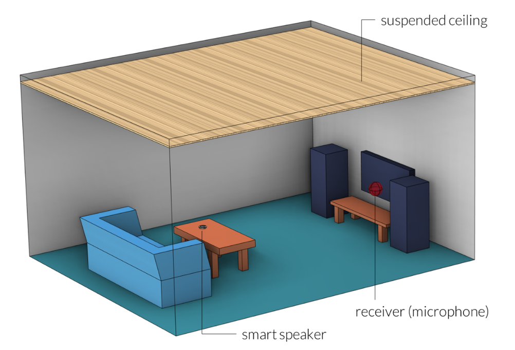
Figure 1. Setup of the problem.
In the current setup, the small smart speaker is modeled by combining pressure acoustics with a lumped representation of the electromechanical components (the Thiele–Small parameters). The lumped Electrical Circuit model is coupled with the Pressure Acoustics, Frequency Domain interface using the Interior Lumped Speaker Boundary feature. For details about this modeling approach, see the Lumped Loudspeaker Driver tutorial model.
A schematic representation of the small smart speaker is given in Figure 2 below. The model includes:
- Front and back air volumes
- The speaker diaphragm (coupled with the lumped element model)
- A perforated mesh
- A vent from the back volume to the exterior
- Thermoviscous boundary layer losses in the narrow regions and small waveguides
The geometry also includes three microphones (modeled with an RCL model), though these are not explicitly used in this tutorial. Note that this is a simplified geometry that can, of course, be extended to a full multiphysics model that involves much more detailed geometry and physics.
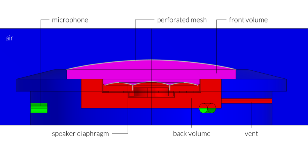
Figure 2. The small smart speaker.
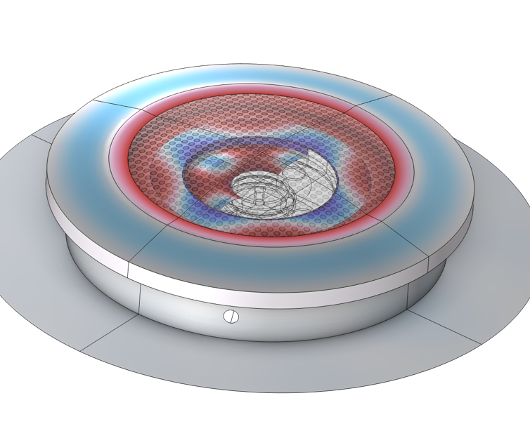
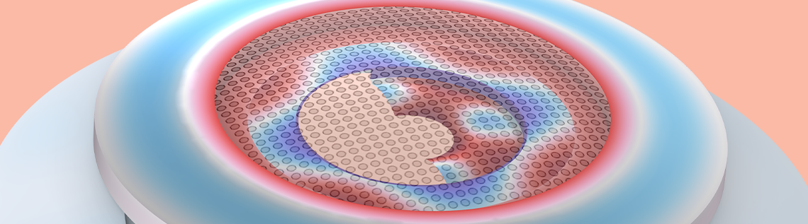
Figure 3. The real part of the acoustic pressure on the speaker surface at 1 kHz.
Combining the Methods
The setup of the model shown here is based on combining the best of the full-wave simulation results with the efficiency of the geometrical acoustics description of ray tracing (when applicable). Here, we show the needed setup for computing the necessary solutions in the low and high frequencies. The concatenation of the high- and low-frequency response is not done in this model, but follows from the model presented in the previously mentioned blog post.
Low Frequency
For the low frequencies, the acoustics of the room and the transducer are solved directly using the Pressure Acoustics, Frequency Domain interface and the Electric Circuit interface. This is set up in Component 2 of the model and solved in Study 2. The latter is used for modeling the electromechanical parts of the transducer. The suspended ceiling is modeled with the Poroacoustics feature. Thermoviscous losses inside the speaker are included using the Narrow Region Acoustics feature for the waveguide structures. For some regions around the voice coil and magnet system where losses are also important, the Thermoviscous Boundary Layer Impedance feature is used.
In this example, the low-frequency regime is solved up to 1200 Hz. The maximum frequency solved for can probably be increased further. To efficiently solve up to this high frequency, we switch to the iterative solver suggestions based on the shifted Laplace method. The model solves about 3.8e6 degrees of freedom (DOFs) and requires about 22 GB of RAM. The model solves from 50 to 1200 Hz in steps of 10 Hz, which takes about 4 h (depending on the hardware). Note that the relative tolerance for the iterative solver needs to be set to 1e-6 to ensure convergence of the coupled FEM and lumped parameter model.

Figure 4. The COMSOL Multiphysics user interface, where the Poroacoustics feature is used to explicitly model the suspended ceiling.

Figure 5. The sound pressure level distribution in the room at 400 Hz.
For another example of using the iterative solver, see the Car Cabin Acoustics — Frequency-Domain Analysis tutorial model.
High Frequency: Two Approaches
For the high-frequencies range, the Ray Acoustics interface is used, but it’s combined with results from full-wave simulations for the representation of the loudspeaker source as well as the angle- and frequency-dependent surface impedance of the suspended ceiling. Two source representations are used and compared.
The first source representation will be referred to as “Release from Point Source”, and it’s in some sense a classical ray-tracing source. The smart speaker radiation characteristics when placed on an infinite baffle (standing on a table) are modeled in Component 1. This is a good example of a submodeling approach that is easily set up in COMSOL Multiphysics®. These results are directly used to define the point source representation in the ray acoustics simulation, using the Release from Exterior Field feature, which is set up and used in Component 3 and solved in Study 3. The setup of the smart speaker in terms of electroacoustic parameters and physics modeled is the same for the source submodel as well as the full (low-frequency) room acoustics model.

Figure 6. The COMSOL Multiphysics® user interface showing the Release from Exterior Field feature that automatically couples the radiation pattern of a full-wave FEM model with a ray-tracing model.
In the second high-frequency ray-tracing approach, the source is not characterized by its far-field radiation characteristic (as a point source), but rather by its near-field characteristics, including details about scattering around the closest table edges. This will be referred to as “Release from Pressure Field”. Here, a full-wave FEM model set up with the Pressure Acoustics, Frequency Domain interface is solved in a sphere surrounding the source (set up in Component 4, with the source solved in Study 4). The idea is that the rays are released from the surface of the sphere in the direction of the acoustics intensity (the “acoustic Poynting vector”) and with the magnitude of the local intensity. This setup is achieved using the Release from Boundary feature in ray acoustics (set up in Component 4, with the source solved in Study 5). The settings can be seen in Figure 7 below. Note that the direction of release is the normalized intensity vector \mathbf{I}/|\mathbf{I}|, and the total (space-dependent) source power is A (\mathbf{I}\cdot\mathbf{n}), where A is the total release area and \mathbf{n} is the surface normal. In both cases, the expressions are wrapped in the bndenv() operator, which ensures that the FEM solution can be mapped to the rays.

Figure 7. The COMSOL Multiphysics user interface settings for the Release from Boundary feature.

Figure 8. An example of the ray release directions and intensity on the surface of the release sphere.
The “Release from Pressure Field” setup combines the full-wave method (near field) with the assumptions relevant for ray tracing. This also sets some restrictions on the use of this formulation for setting up sources. For instance:
- When rays are released using the release from boundary, they are all released at the same time. Because of this, it should be assumed that the sound emanating from the source reaches and leaves every part of the release boundary at the same time. For this to be true, however, the release boundary cannot be placed arbitrarily.
- Because of the restriction mentioned in the previous point, internal reflections in the source domain cannot easily be taken into account. Sound can indeed travel different distances depending on the reflection path taken, which would lead to separate time events at the release boundary and in the impulse response.
- Finally, the time delay (time of flight from the source to the release boundary) is not included in the impulse response computed in ray tracing. The COMSOL® software assumes the release at time to be 0 at the release boundary.
In this model, the near-field sphere radius is set to 0.3 m. This captures diffraction only from the nearest table edges. This size is chosen to prevent making the local full-wave problem too large to solve while still showing the effects of the nearest table edges.
Note that in both ray-tracing models the angle and frequency dependencies of the suspended ceiling absorption are included. The properties are computed in a separate model, shown below.
Properties of the Suspended Ceiling
The properties of the suspended ceiling are included directly in the low-frequency analysis part of the model by modeling the porous layer (using the Poroacoustics feature in the Pressure Acoustics, Frequency Domain interface) as well as the air cavity. In the (high-frequency) ray-tracing simulation, the absorption properties of the suspended ceiling are included as a frequency- and angle-of-incidence-dependent absorption coefficient, \alpha(f,\theta). The absorption data is extracted from a submodel of the suspended ceiling. This model is also available for download here. The model is based on a similar approach to the one used in the Porous Absorber tutorial model. In general, the use of submodeling is a great tool for getting more detailed boundary (and source) conditions for ray-tracing simulations.
The image below shows the absorption surface for the suspended ceiling in the model. The ceiling is made of a 1-cm porous material with a flow resistivity of 20,000 [Pa·s/m2], backed by a 2-cm air cavity. In the ray-tracing model, the angle and frequency dependencies are included by calling an interpolation function with the frequency argument and the angle of incidence variable rac2.wall5.thetai (with the tags for the ray acoustics model 2 and wall condition 5).
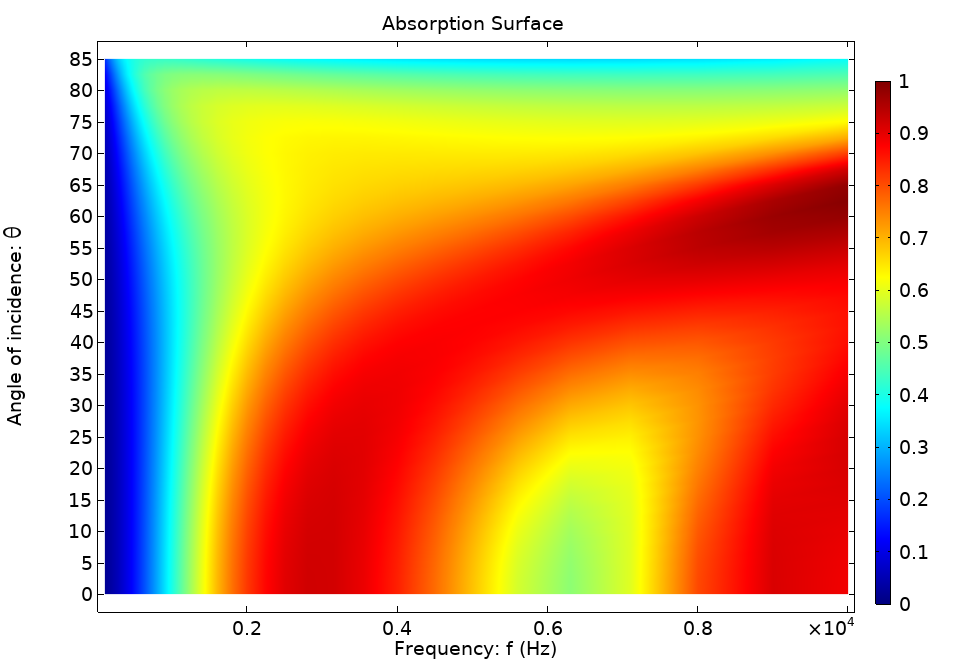
Figure 9. Absorption coefficient surface of the suspended ceiling.
For simplicity, the current model only includes detailed absorption data for the ceiling. The model could very well be extended to include angle- and frequency-dependent absorption data for all boundaries. Detailed scattering data can also be computed from full-wave models, as shown in the Schroeder Diffuser in 2D tutorial model.
Boundary Condition Considerations
The model discussed here has several uses, and various assumptions can be made when it comes to its boundary conditions. These assumptions depend on whether the focus is on pressure acoustics or ray acoustics simulation. Let’s take a closer look at how the modeling considerations and assumptions change depending on the type of simulation.
First, let’s look at some considerations when it comes to pressure acoustics:
- Phase information is modeled here, so it’s generally best to use a frequency-dependent impedance condition.
- Using only the absorption coefficient is typically not accurate at low frequencies.
- The normal impedance of a surface depends on the angle of incidence. So, what value should be used? For room acoustics applications without a clearly defined angle of incidence, using an effective angle is often a good option. For example, as defined in the Porous Layer option in the Impedance condition, the normal impedance is evaluated for an angle of incidence of 50 degrees with the Automatic setting.
- To avoid the abovementioned assumptions, it’s preferable, if possible, to model the actual absorbing surface as done for the suspended ceiling in this model.
In ray acoustics simulations, consider using the:
- Normal versus random incidence absorption coefficient
- Angle-dependent absorption coefficient
- Scattering coefficient
The normal (and random) incidence absorption coefficient, angle-dependent absorption coefficient, and scattering coefficient can be constant or frequency dependent, but your simulation options also depend on the data available.
In addition, for ray acoustics simulation, if the absorption of a wall varies significantly over an octave, consider using a more narrow band representation, like a 1/3- or even 1/6-octave band.
Results
Some selected results from the example model are presented in Figures 10–13. The pressure distribution at 1000 Hz is depicted in Figure 10, and the wave pattern of the solution can be clearly seen. In Figure 11, the location of the rays for the 1000-Hz band is depicted at the same time instance (correcting for the different release times for the two methods), comparing the point source and the release from pressure field description. From the images it’s clear to see that the two methods give different spatial resolutions (ray densities) since the point source only releases to the upper-half space, while the release from the pressure field also releases rays downward (due to diffraction around the table edge). This fact should be taken into account for an even more formal comparison of the methods.
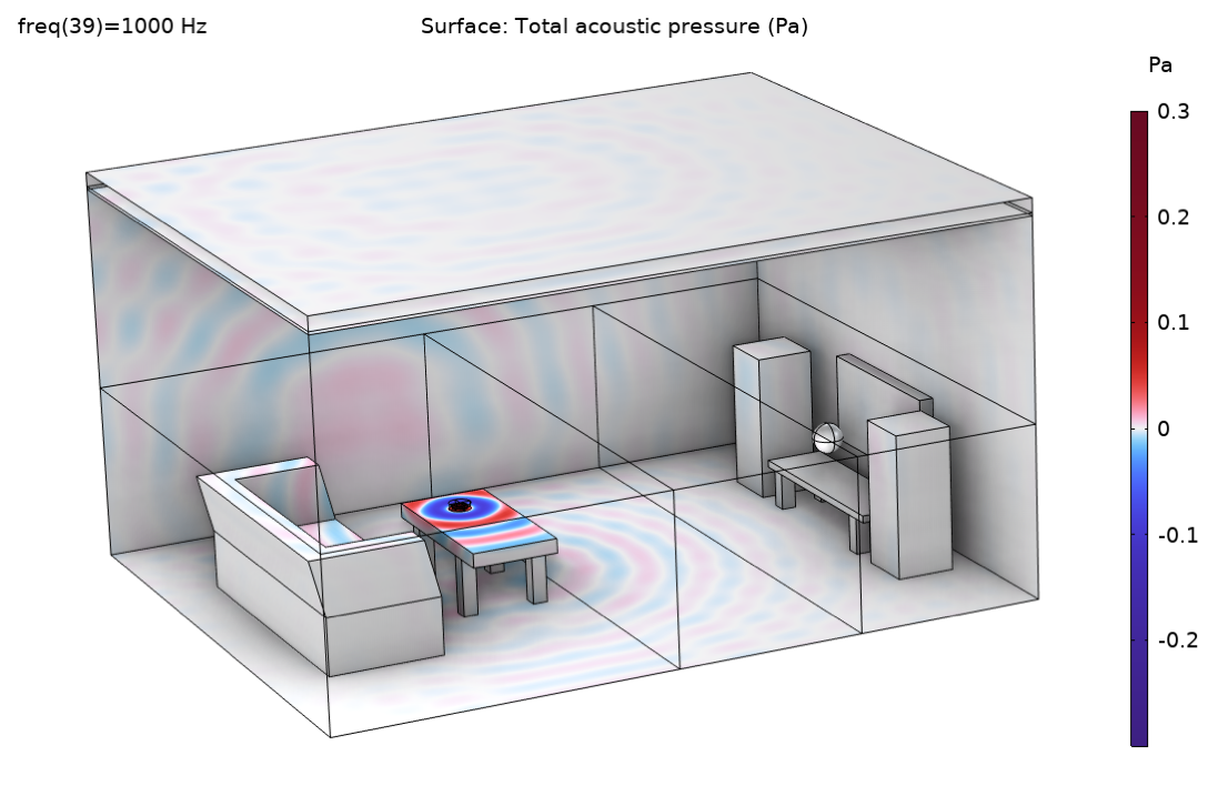
Figure 10. Pressure distribution at 1000 Hz.


Figure 11. A ray plot for the point source (left) and for the release from pressure field (right). Both plots show the 1-kHz band evaluated at 6 ms (approximately corrected for the different definitions of time 0). Note different scales on the color bars for the ray power. In the right-hand image, the acoustic pressure of the near field in the source region is also plotted.
Figures 12 and 13 give a comparison of the methods. The transfer function between the source and receiver is depicted in Figure 12. It plots the fast Fourier transform (FFT) of the impulse response (IR) of the two ray-tracing approaches as well as the full-wave FEM model. There is no smoothing applied to the FEM results, but a 1/3 octave running average filter is applied to the ray-tracing results. The graph shows the same overall behavior. It also shows that there is a strong modal behavior in the room even above the expected Schroeder frequency (vertical line). There seems to be more of a level difference between the two ray acoustics results (blue and red curves). This could be explained by the fact that energy is spread differently by the two source descriptions. Finally, some of the temporal characteristics of the two ray-tracing results are compared in Figure 13. Here, the early decay time (EDT) and reverberation time T20 are compared. The plot shows that there is a significant difference between the two, indicating that the temporal distribution of the energy arriving at the receiver is different for the two models.

Figure 12. Full-wave response and ray acoustics impulse response FFT.

Figure 13. Room acoustic objective metrics comparing the EDT and the T20 reverberation time.
Some of the conclusions discussed here can be refined to extend the analysis carried out in the model. For example, you can choose to use more rays, compare several receiver positions, use a finer frequency resolution for the FEM model, or use a 1/6-octave band for the ray-tracing model. These different options can all be accomplished using the current model. For example, change the number of rays by changing the parameter Nrays or the position of the receiver by changing the parameters xr, yr, and zr.
Next Steps
Further explore the model discussed in this blog post by clicking the button below, which will take you to the Application Gallery.
Additional Resources
- Learn more about rooms acoustics modeling on the COMSOL Blog:
- Check out this related tutorial model:


Comments (2)
Kevin Rivera
July 21, 2023Thanks for information. It’s such a interesting blog. I get some knowledge from it.
Mads Herring Jensen
July 24, 2023 COMSOL EmployeeThank you Kevin! Best regards, Mads