
As part of our solver blog series we have discussed solving nonlinear static finite element problems, load ramping for improving convergence of nonlinear problems, and nonlinearity ramping for improving convergence of nonlinear problems. We have also introduced meshing considerations for linear static problems, as well as how to identify singularities and what to do about them when meshing. Building on these topics, we will now address how to prepare your mesh for efficiently solving nonlinear finite element problems.
Recap of Linear and Nonlinear Static Problems
There are three key points that you should recall from the blog post on meshing considerations for linear static problems. These are:
- A linear static finite element problem will always converge in one Newton-Raphson iteration, regardless of the mesh size.
- You should always start with as coarse a mesh as possible, and either manually refine the mesh or use adaptive mesh refinement to solve finer meshes.
- A mesh refinement study should always be done to assess the accuracy of the results, while monitoring convergence away from any singularities in the model.
When addressing nonlinear problems, we have already learned that even a finite element problem with a single degree of freedom may not converge, even for a problem that has a solution. We have learned several techniques that can address this issue, but have not yet introduced the interplay of the mesh and the nonlinear solver.
Meshing Nonlinear Problems
The single most important thing to keep in mind when meshing nonlinear problems is this:
Even if the problem is well-posed, and even if we have chosen a good solution method, the problem may still fail to converge if the problem is not meshed finely enough in the regions of strong nonlinearities.
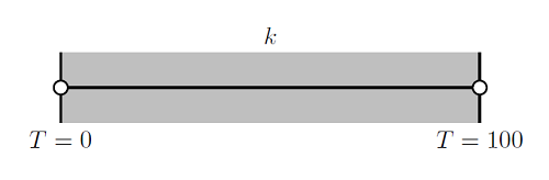
To understand this, let’s take a look at a one-dimensional thermal finite element problem. We will consider a 1 m thick wall with a fixed temperature of T=0 at one end at T=100 at the other, as shown below:
We will examine the solutions to this problem for the different thermal conductivities plotted below:
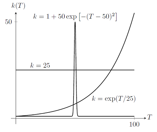
If we plot out the solution for the linear case, k=25, we get:
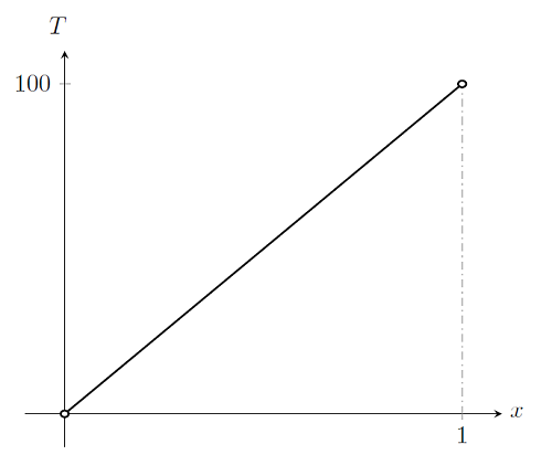
By examination, we see that the solution is a straight line. For this case, the solution can be found by using a single linear element across the entire domain.
Now, if we plot out the case k=\exp(T/25), with elements delineated by dashed lines, we get:
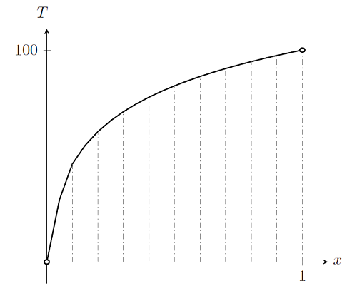
We can see that the solution to this nonlinear problem will require more than a single element across the domain. In fact, regardless of how many elements we use, the polynomial basis function will never perfectly match the true solution. We can successively refine the mesh everywhere in the domain and get closer and closer to the true solution, just as we did for a linear problem.
Finally, if we plot out the case k=1+50\exp\left[-(T-50)^2\right], we get:
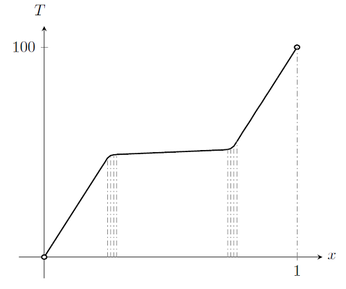
This solution is more complicated. There are clearly regions of the solution where a single element would be almost sufficient to completely describe the solution. Yet, there are regions where the solution varies quite rapidly as a function of position. These regions are around T=50, where there are strong nonlinearities in the material property function. Although the material property function has only one region of strong nonlinearity with respect to temperature, the solution exhibits two regions over the domain where the solution varies rapidly. Only these regions in space require a finer mesh. In fact, the solver might not converge at all if the mesh in these regions is too coarse.
For these types of problems, adaptive mesh refinement becomes highly motivated, since the locations of the gradients in the modeling domain are generally not known ahead of time. Ramping of the nonlinearities in the model is also helpful, since starting with a linear problem will result in a problem that can always be solved, regardless of the mesh. By gradually ramping up the nonlinearity, and performing adaptive mesh refinement iteratively, it is possible to improve model convergence for nonlinear problems.
Summary
Meshing of nonlinear stationary finite element problems is inherently linked with the question of getting a nonlinear model to converge. Convergence rates, and even the possibility of convergence, are dependent on both the solver algorithm used and the mesh. All of the techniques mentioned up to this point: manual and adaptive mesh refinement, choosing of initial conditions, load ramping, nonlinearity ramping, and any combination of these techniques may be needed as you develop more and more sophisticated models. Finally, always keep in mind that a mesh refinement study is needed to assess solution accuracy.
For an example model that incorporates all of the techniques that we have learned about thus far, please see the Cooling and Solidification of Metal model. Mastering these techniques will allow you to quickly and efficiently model nonlinear problems.


Comments (0)