AC/DC Module

Simulate Low-Frequency Electromagnetics and Electromechanical Components

Analyzing electromagnetic systems and processes that encompass the static and low-frequency ranges requires a powerful and flexible simulation tool. The AC/DC Module add-on to the COMSOL Multiphysics® platform provides you with a wide range of modeling features and numerical methods for investigating electromagnetic fields and EMI/EMC by solving Maxwell's equations.

The multiphysics capabilities of the COMSOL® software make it possible to investigate the impact of other physical effects — such as heat transfer, structural mechanics, and acoustics — on an electromagnetics model.

Contact COMSOL
A 3D permanent magnet motor model visualized with copper coils and a rainbow core.

Electric Currents

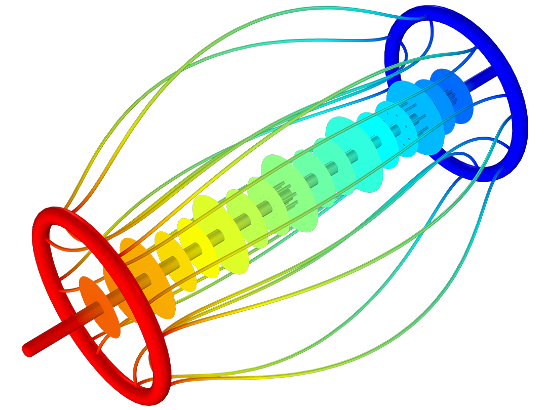
Analyze resistive and conductive devices efficiently by modeling DC, transient, or AC currents. Under static and low-frequency conditions, and when magnetic fields are negligible, modeling electric currents is sufficient for accurate results. The computations, based on Ohm's law, are made very efficient by solving for the electric potential. Based on the resulting potential field, a number of quantities can be calculated: resistance, conductance, electric field, current density, and power dissipation.

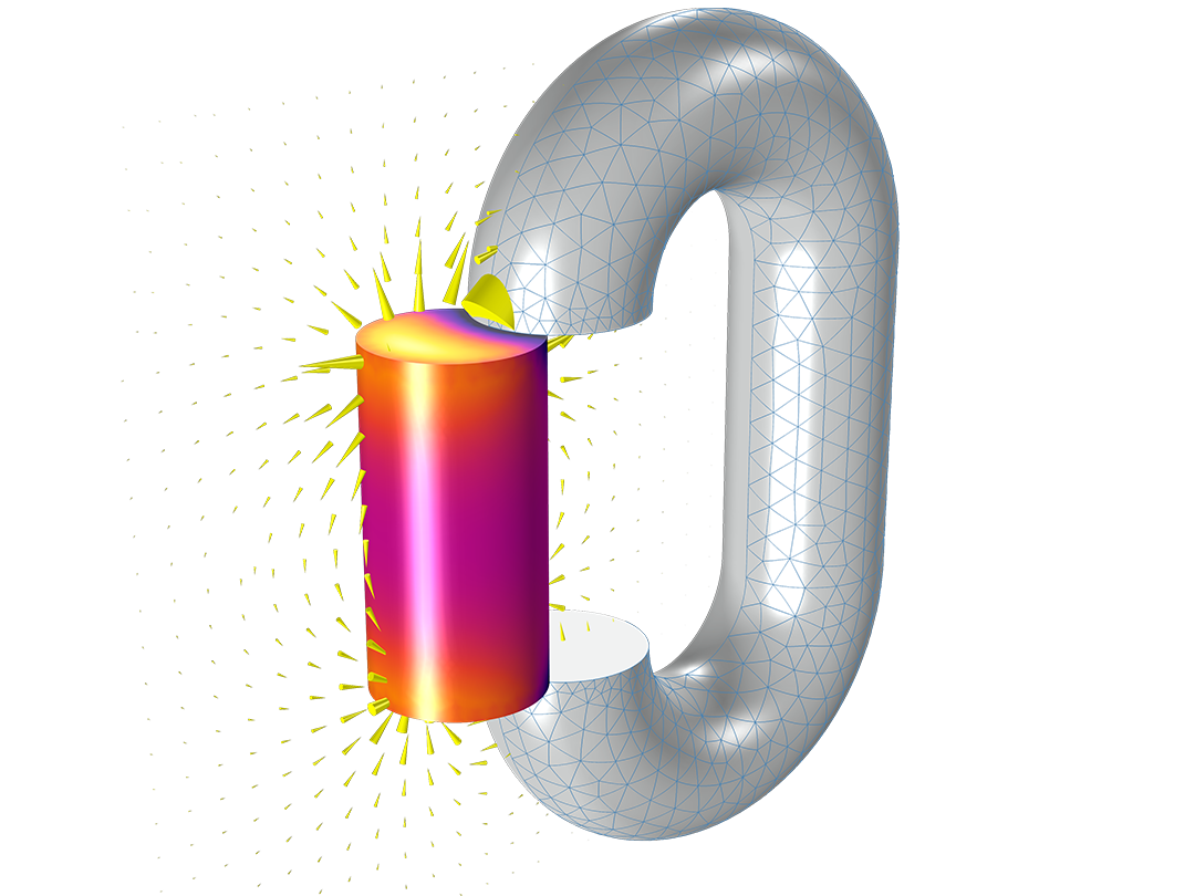
With the AC/DC Module, you can run stationary, frequency-domain, and time-domain analyses, as well as small-signal analysis. In the time and frequency domains, you can also account for capacitive effects.

Electrostatics

Analyze capacitive devices and electrical insulators using electrostatics computations. This approach is applicable for dielectric structures where no currents are flowing and the fields are determined by the electric potential and charge distribution. Both the finite element method (FEM) and boundary element method (BEM) are available to solve for the electric potential, and can be combined for a hybrid finite element–boundary element method. Based on the computed potential field, a number of quantities can be calculated: capacitance matrices, electric field, charge density, and electrostatic energy.

Magnetostatics

Compute magnetostatic fields, parasitic inductances, and forces on coils, conductors, and magnets. You can choose from an extensive material database that includes a wide range of nonlinear magnetic materials, or define your own nonlinear materials. A variety of formulations are available depending on if currents, magnetic materials, or both are present.

Both FEM and BEM are available for magnetostatics in the absence of currents, and can be combined for a hybrid finite element–boundary element method.

For the most general case, where there is both current flow and magnetic materials present, a vector-field formulation allows for electric potential and input currents to be defined, and computes current density distribution, magnetic fields, magnetic forces, power dissipation, and mutual inductances.

Coils can be modeled either explicitly, computing the exact current distribution within each wire, or in a homogenized sense, which is very efficient for coils with many turns. Complex coil shapes are automatically handled by computing the coil current distributions.

Electromagnetic Fields

When modeling cables, wires, coils, solenoids, and other inductive devices, the magnetic field is generated by electric currents flowing in conductive materials. Generally speaking, for time-varying fields with significant induction effects, there is a bidirectional coupling between electric and magnetic fields. In these cases, a vector-field formulation is needed, typically when the skin depth is of the order of the device size, but the wavelength is much larger.

Frequency-domain, small-signal analysis, and time-domain modeling are supported in 2D and 3D. A specialized formulation is available that is particularly suitable for time-domain magnetic modeling of materials with a strongly nonlinear E-J characteristic, such as superconductors.


Rotating Machinery

Built-in functionality for rotating machinery makes it easy to model motors and generators. You can, for example, investigate the behavior of induction or permanent magnet motors, particularly by capturing the eddy current losses that occur within the magnets. In any model that is used for simulating electromagnetic motion, you can examine the rigid or flexible body dynamics under the influence of magnetic forces and torques, induced currents, and mechanical load and spring configurations.

A general-purpose moving mesh functionality makes it possible to model linear motion. This is important for understanding the operation of components involving plungers, such as in magnetic power switches, solenoids, and general actuators.

Electric Circuits

Create lumped systems to model currents and voltages in circuits including voltage and current sources, resistors, capacitors, inductors, and semiconductor devices. Electrical circuit models can also connect to distributed field models in 2D and 3D. Additionally, circuit topologies can be exported and imported on the SPICE netlist format.

Features and Functionality in the AC/DC Module

The AC/DC Module contains specialized features and functionality for the various capabilities presented on this page.

A closeup view of the Model Builder with the Coil node highlighted and a 3D inductor model in the Graphics window.

Built-In User Interfaces

The AC/DC Module provides built-in user interfaces for each of the electromagnetics areas listed above, as well as variations for specific modeling purposes. These interfaces each define sets of domain equations, boundary conditions, initial conditions, predefined meshes, predefined studies with solver settings for steady and transient analyses, as well as predefined plots and derived values.

There are also features that connect the different interfaces, to easily model them together, which can be convenient for inductors, coils, and motors.

A closeup view of the Coil settings and simulation results of a power transformer model in the Graphics window.

Coils

Specialized features are built-in to easily model coils and to convert lumped quantities, like currents and voltages, into distributed quantities, such as current densities and electric fields. Single-conductor and homogenized multiturn coils can be defined in full 3D, 2D, or 2D axially symmetric models. A Part Library, with fully parametric coil and magnetic core shapes, enables a faster model setup when analyzing transformers, inductors, motors, and actuators.

A closeup view of the Model Builder with the Electrostatics, Boundary Elements node highlighted and a tunable capacitor model in the Graphics window.

Unbounded or Large Domains

For accurate modeling of unbounded or large modeling domains, infinite elements are available for both electric and magnetic fields. For electrostatics and magnetostatics modeling, BEM is available as an alternative method for modeling large or infinite regions. Additionally, you can combine BEM with the FEM-based physics interfaces to perform hybrid FEM–BEM simulations.

A closeup view of the Model Builder with the Electric Currents in Layered Shell node highlighted and the electric potential of a heating circuit in the Graphics window.

Thin Structures and Layered Materials

For modeling very thin structures, you can use shell formulations that are available for direct currents, electrostatics, magnetostatics, and induction simulations. Additionally, there is specialized functionality for modeling direct currents in shells with multiple layers. Electromagnetic shell modeling makes it possible to replace the thickness of a thin solid in a CAD model with a physical property of a surface resulting in a much more efficient representation.

A closeup view of the Ampère's Law settings and a 1D plot of the magnetic flux density of a vector hysteresis model in the Graphics window.

Nonlinear Materials

You can choose from a large material database that includes ferromagnetic materials, ferrimagnetic materials, B-H curves, and H-B curves.

Materials can be spatially varying, anisotropic, time-varying, lossy, complex-valued, and discontinuous. It is easy to expand the scope of a simulation with little additional work. You can define your own materials using mathematical expressions, lookup tables, or combinations of both. Full anisotropic hysteresis is supported by means of the Jiles–Atherton material model for quasistatic parametric modeling and full transient analysis. You can even compile your own material model in C-code and link to it as an external material.

A closeup view of the Model Builder with the Loss Calculation node highlighted and a 3D motor model in the Graphics window.

Modeling Losses in Motors and Transformers

Modeling losses in the laminated iron cores and yokes of motors and transformers is important for predicting their efficiency and performance.

In particular, for laminated iron (electrical steel), empirical electromagnetic loss models are important since macroscale Joule heating or induction heating is not able to fully describe the effect causing the losses. At the same time, modeling the laminates individually is often impractical.

The AC/DC Module includes several well-known empirical loss calculation models that give very good loss estimates for only a fraction of the computational effort that a high-fidelity model would take. This includes the effects of magnetic hysteresis and eddy currents, as well as other phenomena that contribute to the losses.

A closeup view of the Stationary Source Sweep settings and simulation results of an inductance matrix in the Graphics window.

Parasitic Inductance and Parameter Extraction

A specialized computational method is available for computing parasitic inductances in PCBs, and is especially efficient for large inductance matrices in 3D. The Magnetic Fields, Currents Only interface is used to calculate the partial contributions from magnetic fields generated by open conductors, reducing modeling complexity.

The magnetic vector potential is used as the dependent variable to compute the magnetic fields generated by currents under the assumption that all regions are nonmagnetic. That is, that the regions have a uniform relative magnetic permeability of "one". The interface can be used with the Stationary Source Sweep feature to sweep over many terminals in one simulation.

Low-Frequency Electromagnetics and Multiphysics

Electromagnetic components affect and are affected by multiple physics phenomena. In COMSOL Multiphysics®, this is no different than modeling a single-physics problem.

A detailed view of a busbar assembly showing the temperature distribution.

Joule Heating and Resistive Heating1

Joule heating (also known as resistive heating) in solids, fluids, shells, and layered shells.

A detailed view of the temperature distribution in a steel billet as it passes through three energized coils.

Induction Heating

Induction heating to model inline induction heaters, and metal processing.

A detailed view of a magnet falling through a copper tube.

Electromagnetic Force and Torque

Finite-element- and boundary-element-based computation of electromagnetic stress, force, and torque.

A detailed view of a loudspeaker driver showing the displacement magnitude.

Lorentz Forces

Current-induced Lorentz forces used as volumetric structural loads for modeling electroacoustic transducers and more.

A detailed view of the electric current streamlines through a contact switch and the temperature distribution.

Electric Contact Resistance

Currents flowing between metallic pieces brought into contact. Combine with thermal2 and mechanical3 contact.

A 1D plot showing hysteresis in a ferroelectric material.

Ferroelectricity

Ferroelectricity functionality used to model a time-varying polarization that may exhibit hysteretic behavior.

A detailed view of a magnetostrictive transducer showing the stress and magnetic field.

Magnetostriction4

Changes to the shape of magnetic materials when subjected to a magnetic field, important for sonar and transformer noise.

A detailed view of a plasma torch model showing the temperature distribution.

Inductively Coupled Plasma5

Inductively coupled plasmas used in semiconductor processing.

A detailed view of an einzel lens model showing particle trajectories and electric potential.

Charged Particle Tracing6

The motion of electrically charged or magnetic particles due to electromagnetic forces.

A detailed view of a DEP filter device showing continuous particle separation.

Dielectrophoresis6

The motion of neutral particles due to electric field gradients.

  1. Does not require the AC/DC Module
  2. Additionally requires the Heat Transfer Module
  3. Additionally requires one of the MEMS Module or Structural Mechanics Module
  4. Additionally requires one of the Acoustics Module, MEMS Module, or Structural Mechanics Module
  5. Additionally requires the Plasma Module
  6. Additionally requires the Particle Tracing Module

Using Third-Party Software with COMSOL Multiphysics®

If you use the MATLAB® software, you can easily drive COMSOL Multiphysics® simulations with MATLAB® scripts and functions. The LiveLink™ for MATLAB® interfacing product lets you access COMSOL® operations directly within the MATLAB® environment and blend them with your existing MATLAB® code.

To make it easy for you to analyze electromagnetic properties of CAD models and electronic layouts, COMSOL offers the ECAD Import Module, CAD Import Module, Design Module, and LiveLink™ products for leading CAD systems as part of our product suite.

You can also synchronize Microsoft Excel® spreadsheet data with the parameters you define in the COMSOL Multiphysics® environment via the LiveLink™ for Excel® interfacing product.

Every business and every simulation need is different.

In order to fully evaluate whether or not the COMSOL Multiphysics® software will meet your requirements, you need to contact us. By talking to one of our sales representatives, you will get personalized recommendations and fully documented examples to help you get the most out of your evaluation and guide you to choose the best license option to suit your needs.

Just click on the "Contact COMSOL" button, fill in your contact details and any specific comments or questions, and submit. You will receive a response from a sales representative within one business day.

Next Step

Request a Software Demonstration