Pipe Flow Module

Design and Analyze Pipe Systems

The Pipe Flow Module, an add-on product to COMSOL Multiphysics®, is used for simulating fluid flow, heat and mass transfer, and acoustics, as well as the mechanical behavior of pipes. In COMSOL Multiphysics®, pipes are represented as 1D segments, significantly reducing the computational resources when compared to meshing and computing flow through 3D pipes. This approach allows you to design and optimize complex pipe applications, including ventilation systems in buildings, pipelines in the oil industry, pipe networks for geothermal applications, and water distribution systems.

In addition to modeling the effects within the pipes, the 1D segments can be embedded in larger 3D volumes to model the effects on the pipes' surroundings. For instance, you can model cooling pipes in engine blocks and injection molds or heating pipes in geothermal applications. The Pipe Flow Module can be combined with other modules from the COMSOL product suite to further expand the multiphysics capabilities for modeling laminar and turbulent flow, solid and shell mechanics, pressure acoustics, and more.

Contact COMSOL
A 3D steering wheel model showing the temperature in the Heat Camera color table.

Efficient Pipe Flow Modeling

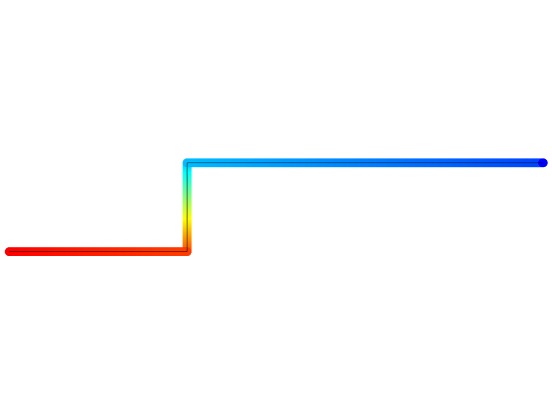
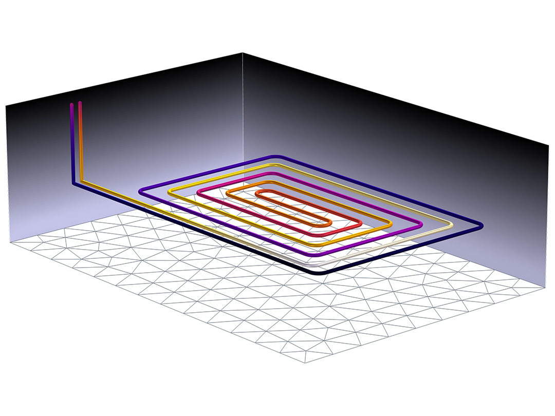
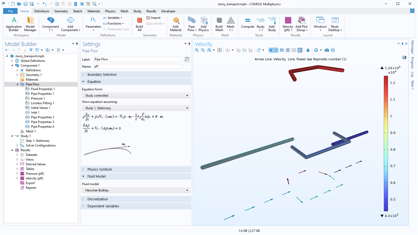
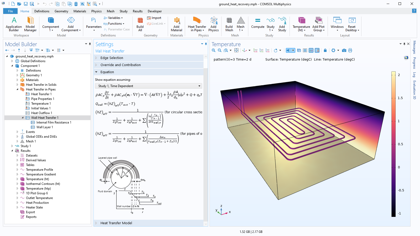
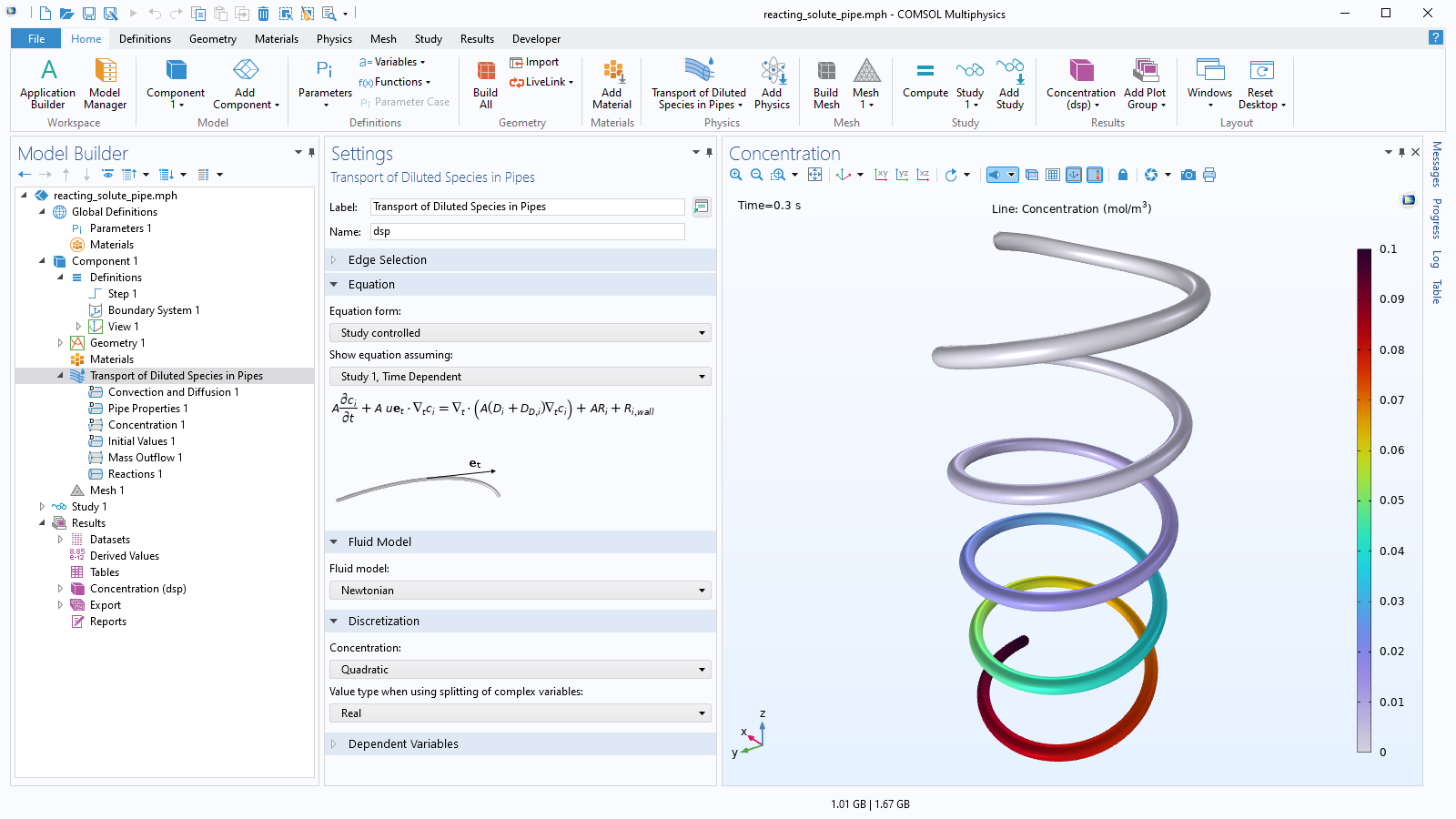
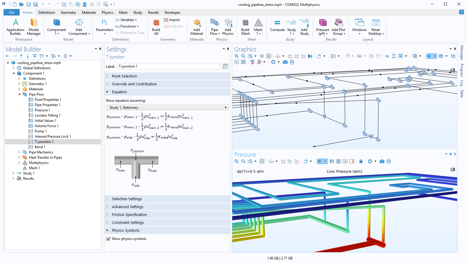
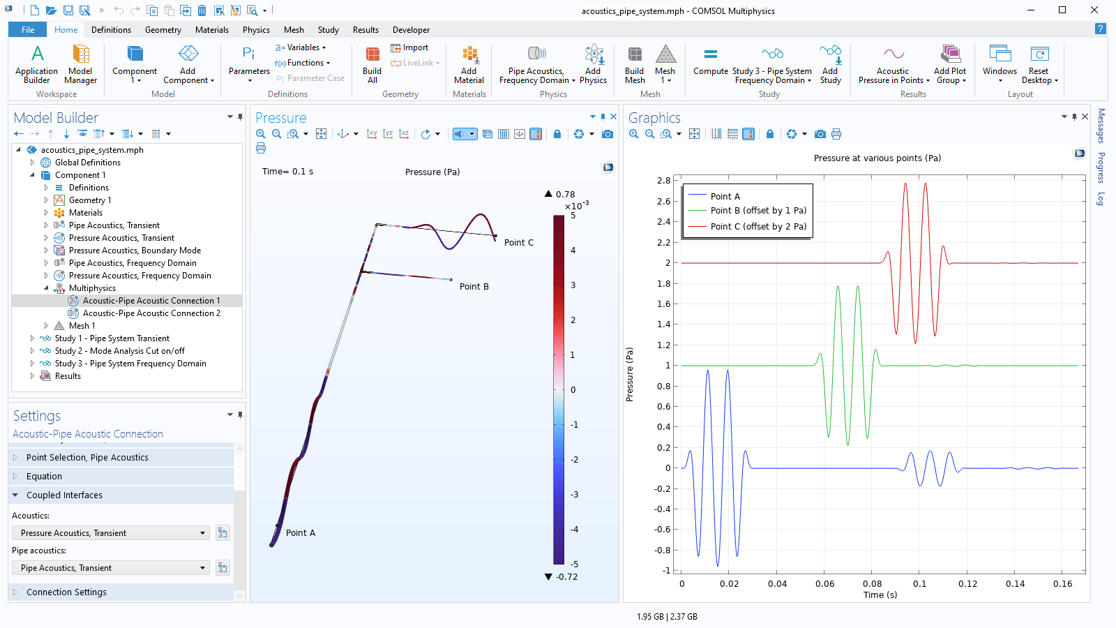
Pipes are objects with high aspect ratios, so using lines and curves rather than volume elements allows you to model piping systems without the need to resolve the complete flow field. The software solves for the cross-section averaged variables along lines and curves in your overall modeling of processes that consist of piping networks, while still allowing you to consider a full description of the process variables within these networks.

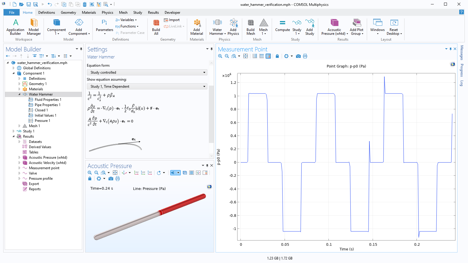
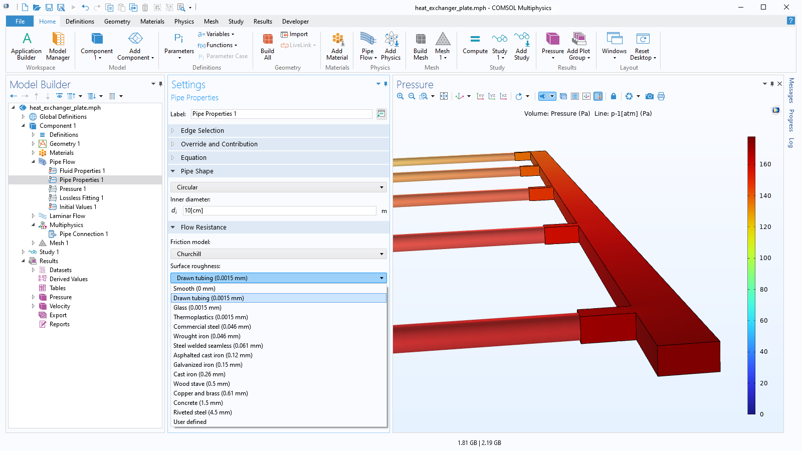
The Pipe Flow Module provides specialized functionality for defining the conservation of momentum, energy, and mass of fluid inside pipes or channels. The pressure losses along the length of a pipe are described using friction factors and relative surface roughness values. Based on this description, you can model the flow rate, pressure, temperature, and concentration in the pipes.

Build Single-Physics and Multiphysics Models

Modeling multiple physics phenomena in COMSOL Multiphysics® is no different than solving a single-physics problem.

A close-up view of a pipe system showing the pressure drop.

Discharging Tanks

Calculate the pressure drop and initial flow rate in tanks.

A close-up view of a heat collector model showing the temperature.

Geothermal Systems

Model geothermal systems and the interactions with their surroundings.

A close-up view of a heat exchanger model showing the pressure distribution.

Heat Exchangers

Model the flow and heat transfer of heat exchangers.

A close-up view of a pipe system showing the acoustic velocity.

Water Hammer Equations

Analyze the propagation of hydraulic transients.

A close-up view of a probe tube microphone model showing the pressure response.

Probe Tube Microphones

Investigate microphone sensitivity with 1D and 3D couplings.1

A close-up view of a steering wheel model showing the temperature.

Cooling Systems

Model the cooling of injection-molded parts.

A close-up view of a pipe network model with two heat producers.

Pipe Networks

Optimize the layout of pipe networks to maximize efficiency.2

A 1D plot showing the insulation in a pipeline.

Insulation

Simulate oil transportation in pipelines.

A close-up view of a heat exchanger model showing the pressure and velocity.

Laminar and Turbulent Flows

Combine pipe flow domains with 3D fluid domains for both laminar and turbulent flows.3

A close-up view of a pond loop model showing the temperature.

Nonisothermal Flow

Solve flow, pressure, and temperature simultaneously.

  1. Requires the Acoustics Module
  2. Requires the Optimization Module
  3. Requires the CFD Module or Heat Transfer Module

Features and Functionality in the Pipe Flow Module

The Pipe Flow Module is a complement to the other add-on modules with fluid flow capabilities.

A close-up view of the Pipe Flow settings and a slurry transport model in the Graphics window.

Pipe Flow

The Pipe Flow Module contains built-in physics interfaces that define the conservation of the momentum, energy, and mass of fluid inside a pipe or channel system. The Pipe Flow interface is used for computing the velocity and pressure fields in pipes and channels of different shapes. It approximates the pipe flow profile by 1D assumptions in curve segments or lines. These lines can be drawn in 2D or 3D and represent simplifications of hollow tubes.

For users of the CFD Module and Heat Transfer Module, a Pipe Connection multiphysics coupling is available for cases where piping systems open up to a larger fluid volume. This feature couples a 1D pipe segment (modeled with the Pipe Flow interface) with a 3D single-phase flow body to provide continuity in mass flux and pressure, regardless of direction.

A close-up view of the Model Builder with the Wall Heat Transfer node highlighted and a geothermal system in the Graphics window.

Heat Transfer

The Heat Transfer in Pipes interface is used for modeling heat transfer by conduction and convection in pipes and channels of different shapes, where the fluid velocity and pressure are known a priori. The interface uses 1D energy balance to determine the temperature profiles in curve segments or lines. These lines can be drawn in 2D or 3D and represent simplifications of hollow tubes. Functionality for modeling wall heat transfer, including multilayer walls and cladding, is included as an option. The Nonisothermal Pipe Flow interface extends this physics interface by providing equations to compute the velocity and pressure fields when they are unknown. More extensive descriptions of heat transfer, such as 3D turbulent flow models or problems involving surface-to-surface radiation, can be found in the Heat Transfer Module.

A close-up view of the Fluid-Pipe Interaction settings and a pipe network model in the Graphics window.

Mechanical Analysis of Pipes

The Pipe Mechanics interface is used for computing stresses and deformations in pipes with loads such as internal pressure, junction forces, and axial drag forces. The Fluid-Pipe Interaction, Fixed Geometry multiphysics coupling can be used to model flow-induced loads in pipes, such as pressure and drag forces, centrifugal forces in curved pipes, and fluid loads at bends and junctions. With the add-on Structural Mechanics Module, a Structure-Pipe Connection multiphysics node is available to couple the Structural Mechanics interfaces with the Pipe Mechanics interface.

A close-up view of the Model Builder with the Water Hammer node highlighted, the corresponding Settings window, and a pipe system in the Graphics window.

Water Hammer Analysis

When a valve is closed rapidly in a pipe network, it gives rise to a hydraulic transient known as a water hammer. The propagation of these hydraulic transients can, in extreme cases, cause overpressures that lead to failures in pipe systems. The Water Hammer interface in the Pipe Flow Module can be used for modeling compressible flow brought about by rapid hydraulic transients by taking the elastic properties of both the fluid and high wall into account.

A close-up view of the Model Builder with the Transport of Diluted Species in Pipes node highlighted and a pipe model in the Graphics window.

Chemical Species Transport

With its capabilities for modeling the transfer of chemical compounds diluted in fluids flowing through thin pipes, the Pipe Flow Module allows for complex chemical reaction modeling. This can include mass transfer, chemical kinetics, heat transfer, and pressure drop calculations in the same model.

The Transport of Diluted Species in Pipes interface solves a mass balance equation for pipes in order to compute the concentration distribution of a solute in a dilute solution, considering diffusion, dispersion, convection, and chemical reactions.

A close-up view of the Pipe Properties settings and a heat exchanger model in the Graphics window.

Friction Models

The flow, pressure, temperature, and concentration fields across the pipe cross sections are modeled as cross-section averaged quantities, which only vary along the length of the pipes and channels. For single-phase flow, the pressure losses along the length of a pipe or in a pipe component are described using friction factor expressions.

The available friction models for Newtonian fluids include Churchill, Wood, Haaland, Von Karman, and Swamee-Jain. When one of these friction models is selected, the surface roughness data can be selected from a predefined list.

For non-Newtonian fluids in tubes of circular cross sections, the Irvine and Stokes friction models are available for Power-law fluids, Darby is available for Bingham fluids, and Swamee-Aggarwal for Herschel-Bulkley fluids. For non-Newtonian fluids in tubes of noncircular cross sections, a value or expression can be entered for the Darcy friction factor.

A close-up view of the T-junction settings and two Graphics windows showing a pipeline network model.

Junctions, Inlets, Valves, Bends, and Pumps

To account for correlations of sudden pressure change for common elements of pipe networks, the Pipe Flow Module includes features to introduce additional pressure losses due to irreversible turbulent friction at a point associated with bends, valves, pumps, or contractions or expansions in a pipe system. An Inlet feature is available to set the velocity, volumetric flow rate, or mass flow rate inlet conditions that describe the fluid flow.

In addition to the continuous frictional pressure drop along pipe stretches, pressure drops due to momentum changes in components are computed through an extensive library of industry-standard loss coefficients. Friction losses in pipe junctions are characterized by many variables, and the geometries may differ by angles, cross sections, and the number of branches. The Pipe Flow Module offers a variety of junction types that can act as a split or merger, such as T-junction, Y-junction, and N-way junction, to specify additional losses due to irreversible turbulent friction.

A close-up view of the Pipe Flow settings and a pipeline system model in the Graphics window.

Non-Newtonian Fluids and Multiphase Flow

For single-phase flow modeling, the fluid can be characterized according to its response and the actions of shear stresses. Newtonian fluids have a linear relation between shear rate and shear stress. In the case of non-Newtonian fluids, the relationship between shear rate and shear stresses can be nonlinear. The Bingham plastic fluid model is available to describe viscoplastic fluids that have a yield stress. For shear-thinning fluids and shear-thickening fluids, the Power law fluid model is available. The Herschel-Bulkley fluid model is used to describe the rheological behavior of non-Newtonian fluids and to simulate the flow of fluids exhibiting viscoplastic behavior. With the non-Newtonian fluid models, you can model phenomena such as water and mineral suspension.

The Newtonian fluid type also has two gas–liquid options: the Gas-Liquid, friction factor multiplier, which modifies the single-phase Newtonian Darcy friction factor; and the Gas-Liquid, effective Reynolds number, which uses an effective, adjusted viscosity to calculate the Reynolds number in the pressure loss calculations. Two-phase gas–liquid flow is a common phenomenon in the nuclear, oil & gas, and refrigeration industries, where gas mixtures are transported in pipe systems.

A close-up view of the Model Builder with the Acoustic-Pipe Acoustic Connection node highlighted and a pipe system in the Graphics window.

Acoustic Wave Propagation

The propagation of acoustic waves along flexible pipes is a contributing factor to the design, planning, and building of these networks. The Pipe Acoustics interfaces can be used for 1D modeling of the propagation of sound waves in pipe systems.

With the Acoustics Module add-on, you can perform 3D-to-1D acoustics analyses in both the frequency and time domains. To compute the propagation of acoustic waves in fluids at quiescent background conditions, the Pressure Acoustics, Frequency Domain interface is available for time-harmonic analyses and the Pressure Acoustics, Transient interface is available for transient simulations.

The Acoustics Module also provides an Acoustic-Pipe Acoustic Connection multiphysics coupling to combine the Pressure Acoustics interfaces with the Pipe Acoustics interfaces in both frequency- and time-domain simulations. The coupling is defined between a point in the pipe acoustics interface and a boundary in the pressure acoustics interface.

Every business and every simulation need is different.

In order to fully evaluate whether or not the COMSOL Multiphysics® software will meet your requirements, you need to contact us. By talking to one of our sales representatives, you will get personalized recommendations and fully documented examples to help you get the most out of your evaluation and guide you to choose the best license option to suit your needs.

Just click on the "Contact COMSOL" button, fill in your contact details and any specific comments or questions, and submit. You will receive a response from a sales representative within one business day.

Next Step

Request a Software Demonstration