
When modeling a manufacturing process, such as the heating of an object, it is possible for irreversible damage to occur due to a change in temperature. This may even be a desired step in the process. With the Previous Solution operator, we can model such damage in COMSOL Multiphysics. Here, we will look at the “baking off” of a thin coating on a wafer heated by a laser.
Heating a Wafer to Remove a Thin Film of Material
Let’s consider a wafer of silicon with a very thin layer of material coated on the surface. This thin film may have been introduced in a previous processing step, and we now want to quickly “bake off” this material by heating the wafer with a laser. The wafer is mounted on a spinning stage while the laser heat source traverses back and forth over the surface.
We will consider a layer of material that is very thin compared to the wafer thickness. We can thus assume that the film does not contribute to the thermal mass of the system, nor will it provide any additional conductive heat path. However, this coating will affect the surface emissivity. If the coating is undamaged, the emissivity is 0.8. Once the coating has baked off, the emissivity of that region of the wafer will change to 0.6. This will alter both the amount of heat absorbed from the laser heat source and the heat radiated from the wafer to the surroundings.
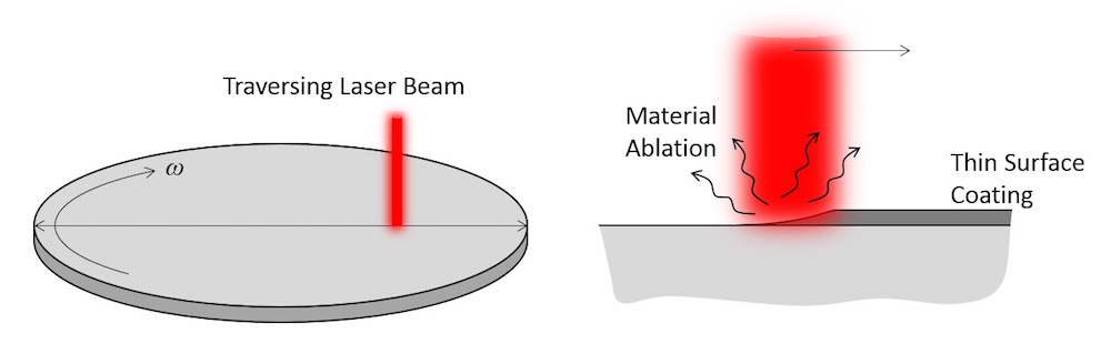
A laser beam traversing over a rotating wafer ablates a thin surface coating when the temperature is high enough.
We will not concern ourselves too greatly with the process by which the coating is removed from the wafer. Although the actual process may include phase change, melting, boiling, ablation, and chemical reactions, we are, in this case, dealing with a very thin layer of material. Thus, we can simply say that once the temperature of the wafer surface exceeds 60°C, the coating immediately disappears. Under the assumption of very fast dynamics of the material removal process relative to the heating of the wafer, this is a valid approach.
Implementation of the Material Removal Model
We will begin with the previously developed model of a rotating wafer exposed to a moving heat source. An additional boundary equation will be added to our existing model. Hence, we need to model this in a coordinate system that moves with the rotation of the wafer.
The equation we add will track the surface emissivity on the top boundary of the wafer. The Previous Solution operator is used since we simply want to change the surface emissivity once the temperature gets above the specified value and leave it otherwise unchanged. We have already introduced the use of the Previous Solution operator in a previous blog entry. We will now focus more specifically on modeling the removal of the film from the wafer surface.
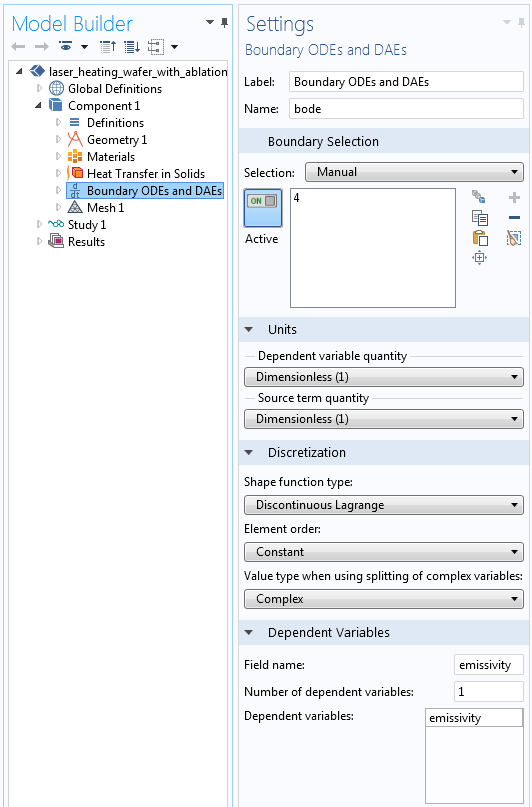
The settings for the Boundary ODEs and DAEs interface. Note the shape function settings.
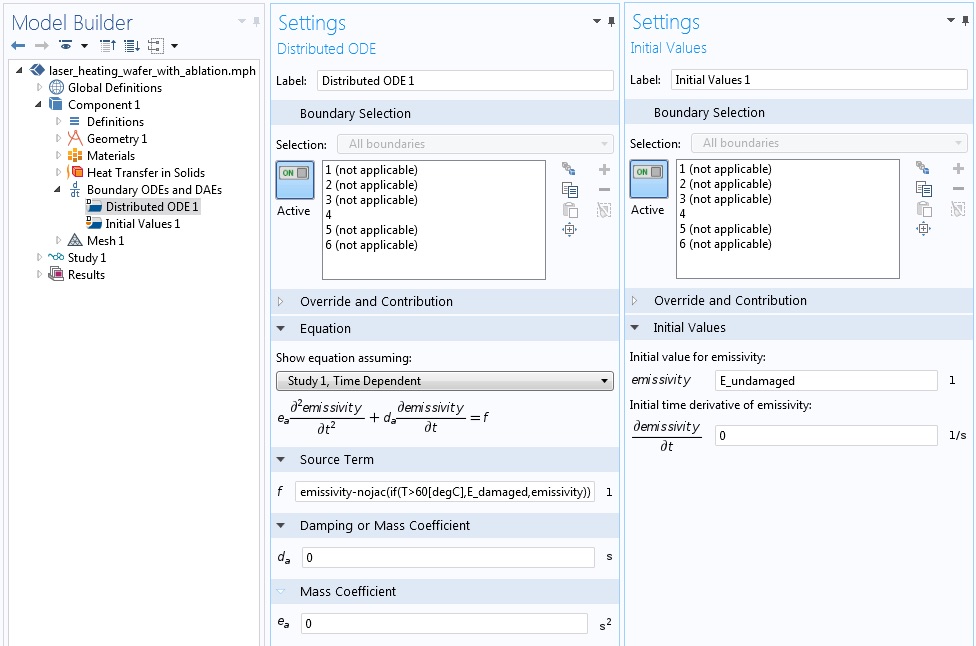
The domain settings and initial values settings for the Boundary ODEs and DAEs interface, which models the emissivity of the surface of the wafer.
The settings for the Boundary ODEs and DAEs interface are shown above. Note that a Constant Discontinuous Lagrange discretization is used to solve for the field “emissivity”, the surface emissivity. This discretization is equivalent to saying that the emissivity will have a constant value over each element and that the field can be discontinuous across different elements. We are assuming that the film is either present or not present, so the surface emissivity will have two discrete states. The initial value of the field variable is the undamaged value of the surface emissivity.
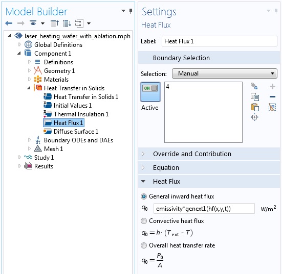
The settings for the Heat Flux boundary condition use the computed surface emissivity.
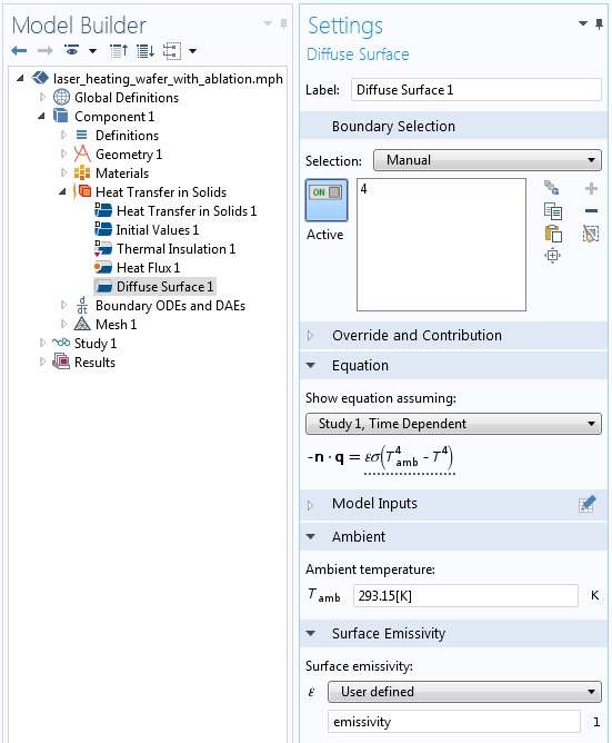
The settings for the Diffuse Surface boundary condition use the computed surface emissivity.
The computed surface emissivity is used in two places within the Heat Transfer in Solids interface, as shown above. The applied Heat Flux boundary condition and the radiation of ambient temperature via the Diffuse Surface boundary condition both reference the emissivity field.
Since the surface emissivity is constant across each element, a finite element mesh size of 0.3 mm is used to obtain a smoother representation of the damage field. Also, the relative solver tolerance is set to 1e-6.
The results of the simulation are depicted in the animation below. As the temperature rises, certain portions of the wafer surface rise above the ablation temperature and the surface emissivity changes. The process is complete once the entirety of the wafer surface has been heated above the desired temperature.
An animation of the temperature field of the laser heating the rotating wafer (left). The dark gray color indicates the damage zone (right).
Summary
We have demonstrated how to model an irreversible change in the state of a material. In this case, we have analyzed the removal of a thermodynamically negligible thin layer of material from the surface of a wafer and modified the resultant surface emissivity as a consequence. The technique outlined here for using the Previous Solution operator can also be used in many other cases. What comes to your mind?
If you are interested in downloading the model related to this article,
it is available in our Application Gallery.


Comments (8)
天然 马
June 17, 2020案例库里没有提供模型文件,请问是否可以分享下文中的案例?
Lyubo
July 19, 2020Is there limitation how thin the coating can be? Can it be also thick instead of thin?
Bob Davis
March 8, 2021Hello
Can you please tell me what laser profile did you use?
And how did you change the space in Genxt 2?
Also, how much did you assume the amount of E_undamage?
And why does the (Distributed ODE 1) section warn me of the value you defined when I paste it?
Walter Frei
March 8, 2021 COMSOL EmployeeThis article has be superseded by:
https://www.comsol.com/blogs/how-to-use-state-variables-in-comsol-multiphysics/
and by updates to this example:
https://www.comsol.com/model/laser-heating-of-a-silicon-wafer-13835
Note that these examples are really more meant to be examples of functionality within the software, and are not meant to be definitive suggestions about how to model any specific case.
Bob Davis
April 9, 2021Thank you dear Mr. Walter Frei
Songcai Han
August 20, 2021It works well for homogeneous materials. However, it is found that the solutions at previous step cannot be accurately recorded for a model with heterogeneous material properties, no matter what shape function you set in ODE. So, are there other solutions?
Hassan Mohamed Osman
August 29, 2024Dear Walter Frei,
Is it possible to provide the tutorial .mph file for the above discussion? I am having difficulties generating your results by looking at your previous posts at the same time. I edited the laser heating tutorial to include the previous solution operator and the emissivity as you shown above but I could not visualize the damage zone. I am getting the following error(Previous-component solver failed.
Size of sparse matrices disagree.
Last time step is not converged.)Please help. thanks
Walter Frei
August 30, 2024 COMSOL EmployeeThis article has be superseded by:
https://www.comsol.com/blogs/how-to-use-state-variables-in-comsol-multiphysics/
and by updates to this example:
https://www.comsol.com/model/laser-heating-of-a-silicon-wafer-13835
We suggest you instead use that approach.