Track Charged Particles and Particles in Fluid Flow with Simulation

Electron trajectories passing through three gray electrodes and surrounding isosurfaces of the electric potential.

Charged Particle Tracing

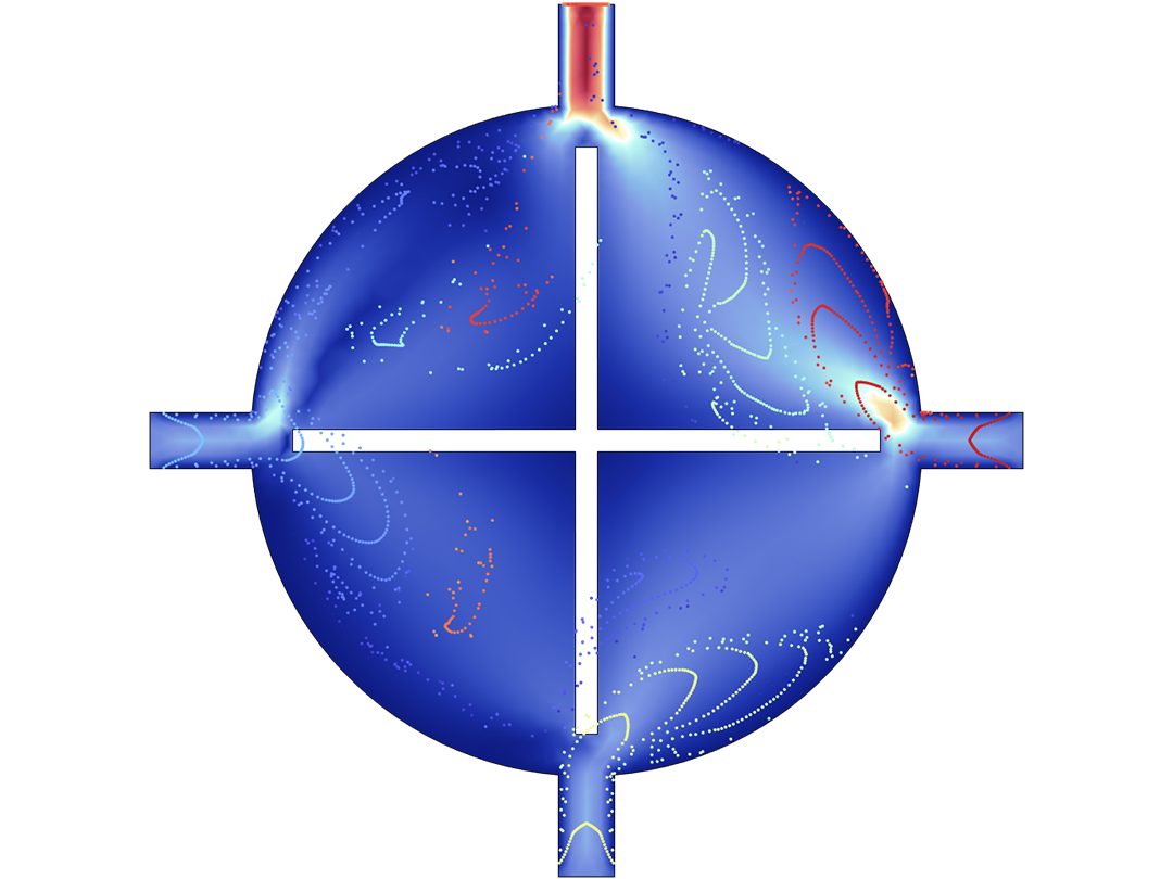
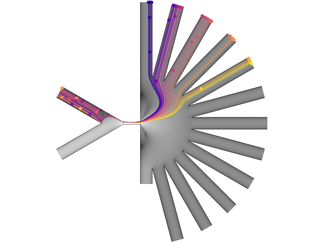
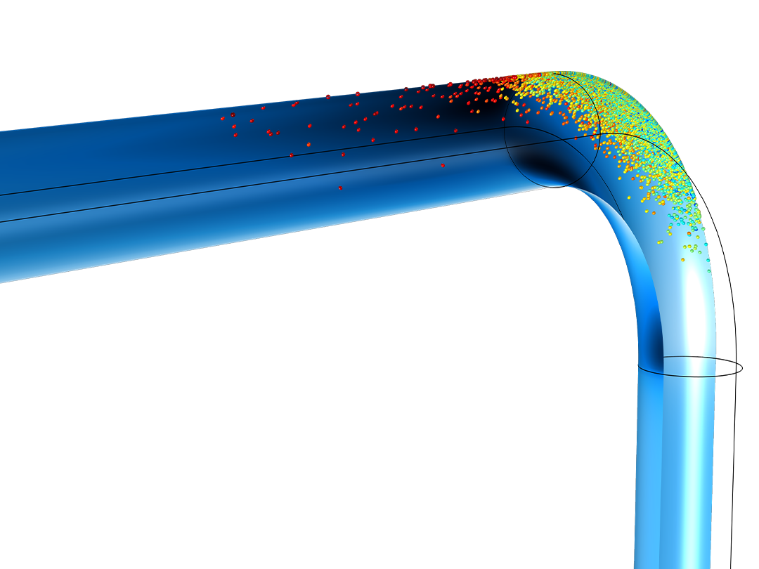
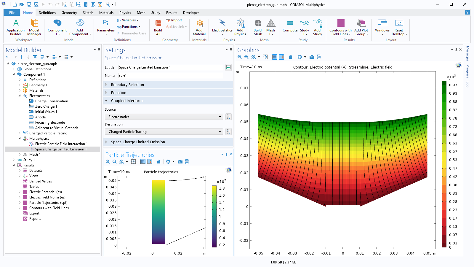
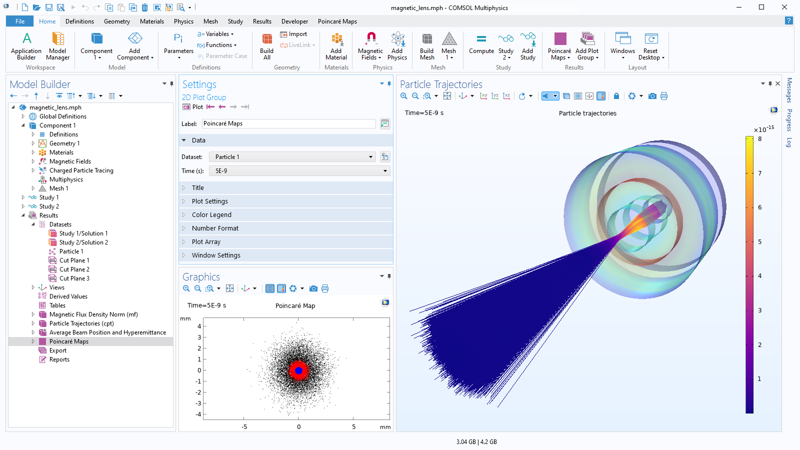
Accurately predicting the motion of ions or electrons in applied fields is essential to the design of spectrometers, electron guns, and particle accelerators. The applied fields might be user defined or taken from a previous analysis. Such fields can be stationary, time dependent, or solved for in the frequency domain. Any number of different fields can be applied, enabling stationary and time-harmonic fields to be superposed in the same simulation.

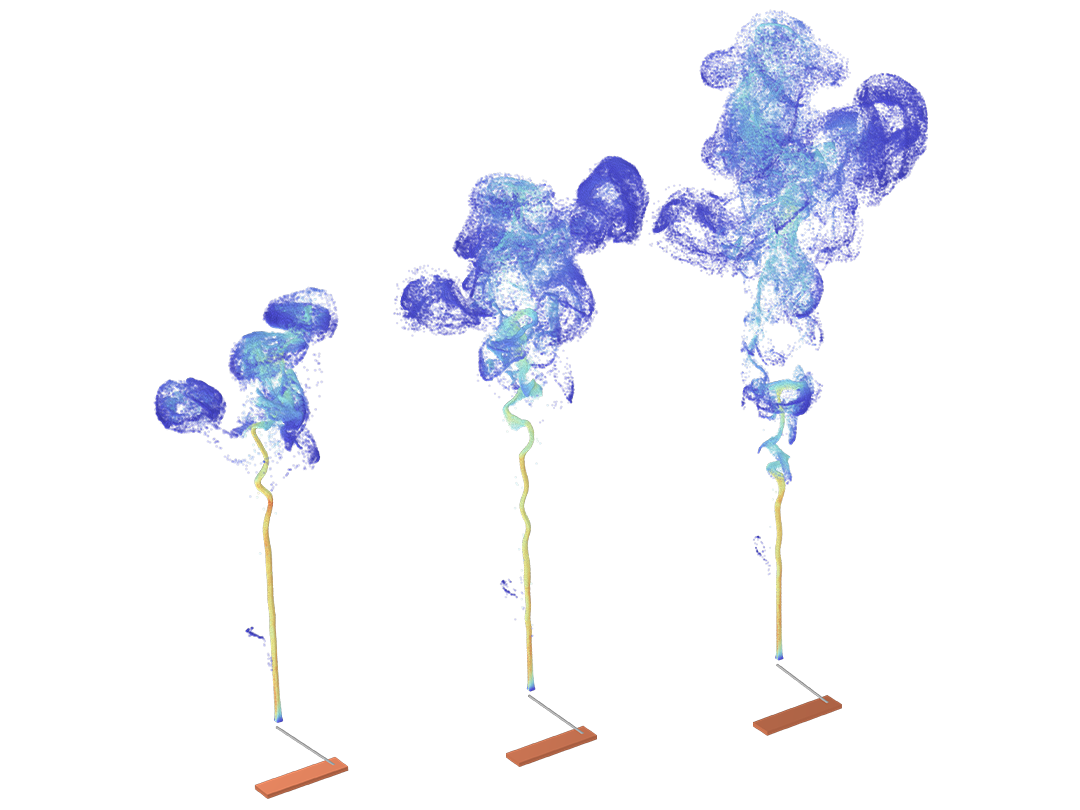
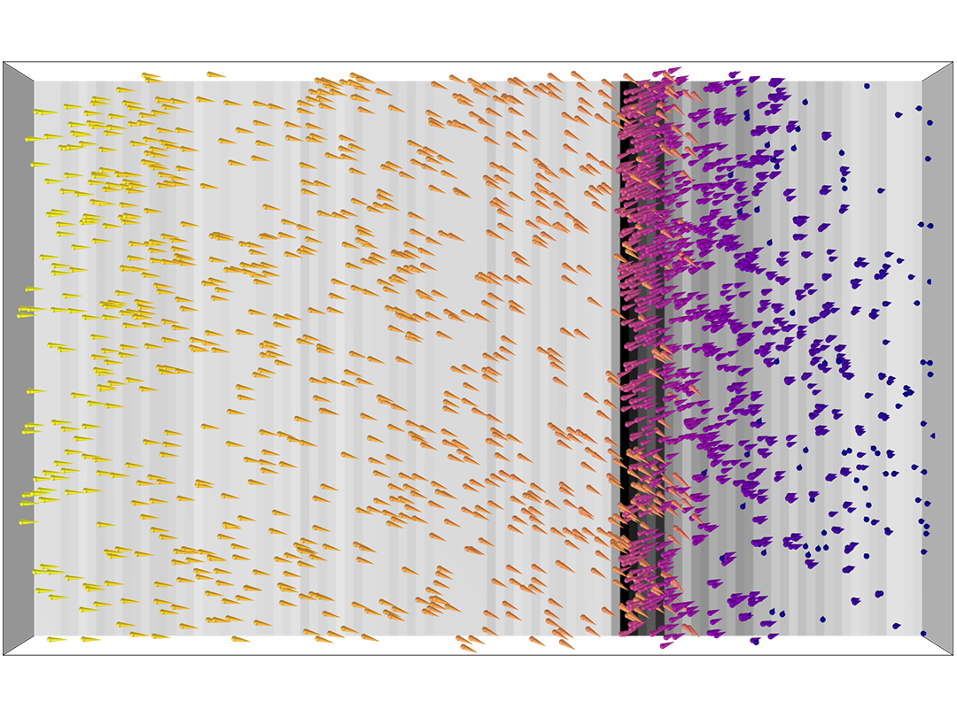
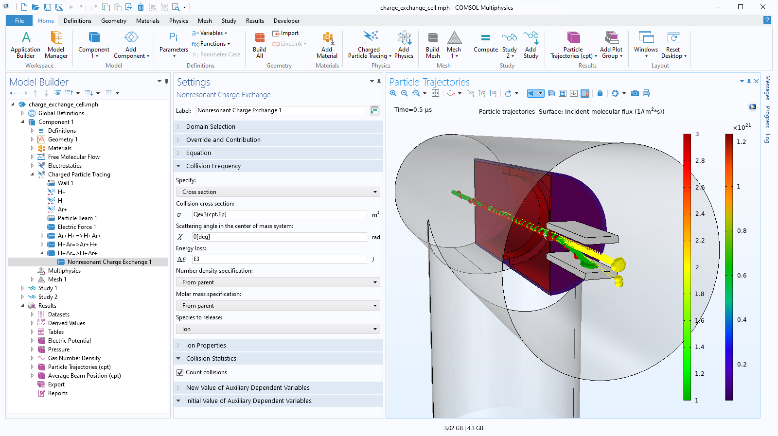
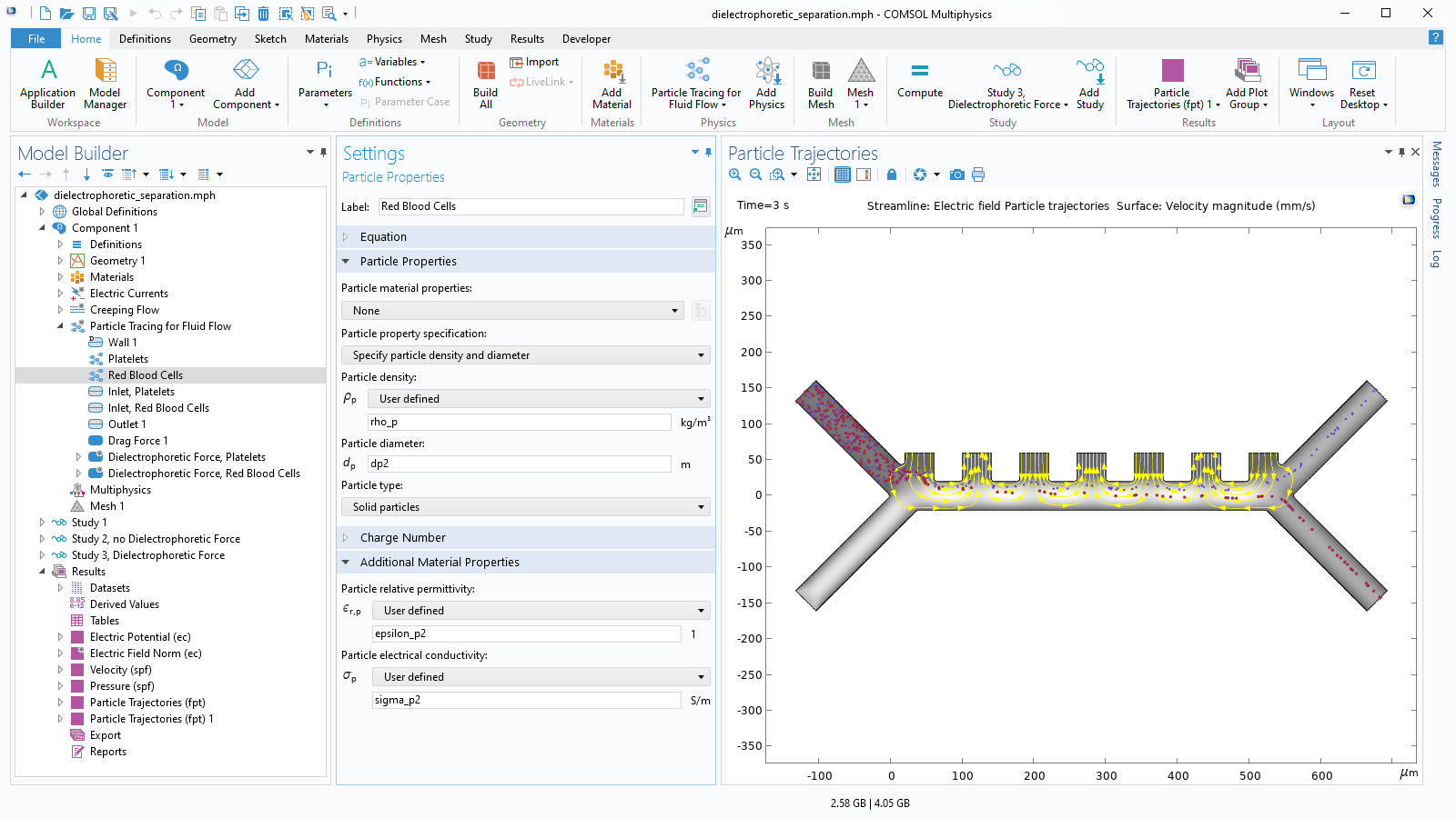
Particle motion seldom takes place in a perfect vacuum. Any particle tracing model can be turned into a Monte Carlo collision model, giving the particles some chance to collide with molecules in the surrounding gas. Such collisions might cause particles to change direction or even undergo reactions such as ionization and charge exchange.

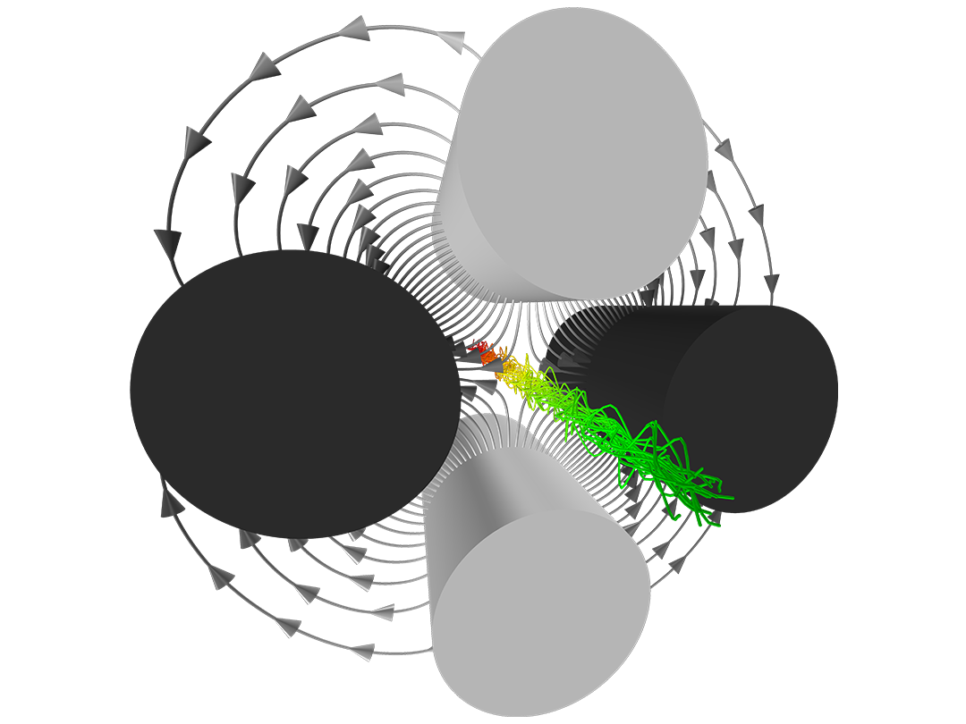
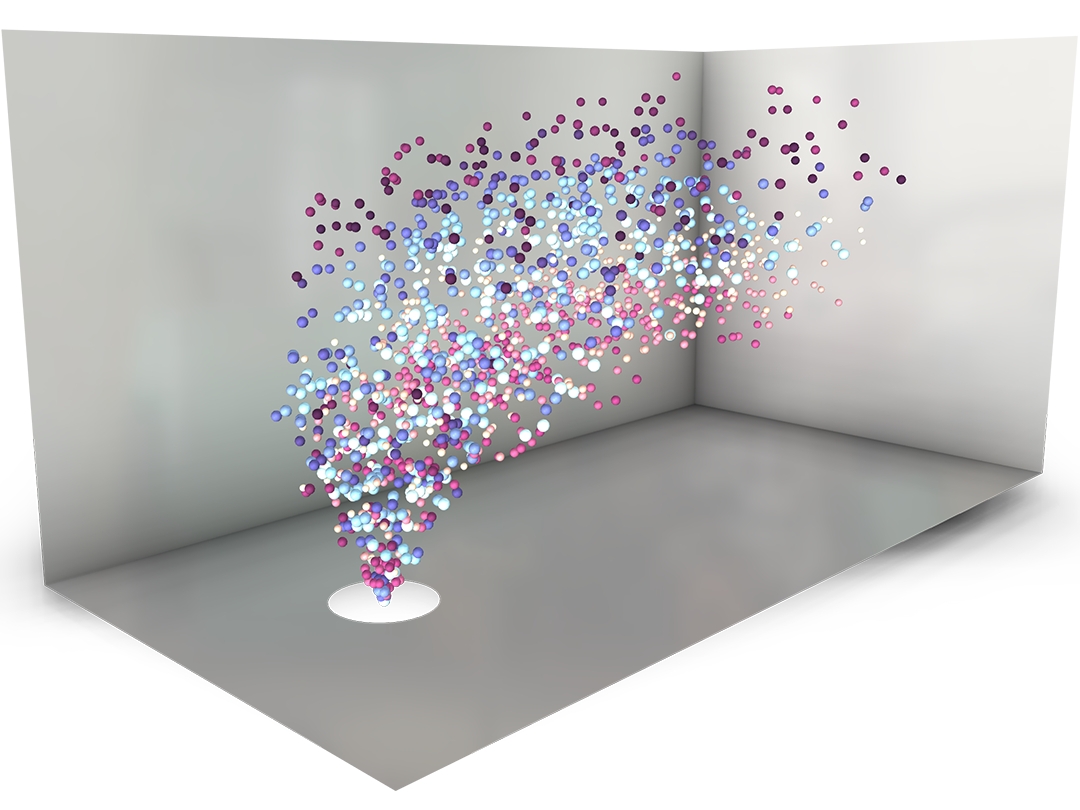
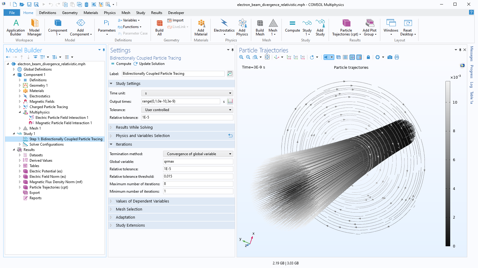
The simplest charged particle tracing models involve unidirectional (one-way) coupling, where the fields are solved and then used to define forces on the particles. If the charged particles are in a beam of sufficiently high current, it might then be necessary to consider the bidirectional (two-way) coupling, where the particles can perturb the field. Built-in analysis types are available to conveniently set up bidirectionally coupled models.

Particle Tracing for Fluid Flow

The dispersion and evaporation of airborne water droplets, the migration of biological cells in a lab-on-a-chip device, and the impact of sediment on the walls of oil and gas pipelines are all examples of particle tracing for fluid flow.

For particles in a fluid, the most important forces are often drag and gravity. Depending on the application, additional forces such as lift, electric, magnetic, thermophoretic, and acoustic radiation forces may also be applied. The particle motion might involve a random component if the fluid is turbulent or if the particles are small enough that Brownian motion is significant.

Particles might all have the same size, or they may be sampled from a size distribution. Optionally, the heating or cooling of particles due to their surroundings can be modeled, and particles can be made to gain or lose mass as they propagate.

For larger particles, a full inertial treatment of the equations of motion accurately predicts how each particle will accelerate in the surrounding fluid. The fluid velocity can be typed in manually or taken from a previous analysis. Some approximate methods are also available to significantly reduce simulation time, especially for small particles with negligible inertia.

Unidirectional coupling analyses can be performed to trace particle motion in dilute flows, and bidirectional coupling analyses can be performed for models where the fluid motion is expected to be affected by the presence of the particles.

Three incense sticks at different times showing the produced smoke as blue-purple particle trajectories, where the plume of smoke grows from the left stick to the right stick.

Mathematical Particle Tracing

As an alternative to the built-in functionality for charged particle tracing and particle tracing for fluid flow, the Particle Tracing Module includes a general-purpose interface for solving any particle equation of motion that might be specified. Any number of user-defined release features, boundary conditions, domain conditions, and forces can be included.

The options for specifying forces on the particles include using Newton's second law of motion or, indirectly, by specifying a Lagrangian or a Hamiltonian for the particle system.

Particle motion can also be traced in domains that move or deform over time. For domains undergoing simple rotation, the motion may instead be simulated in the rotating reference frame by introducing pseudoforces.

What Can Be Modeled with the Particle Tracing Module

Simulate the behavior of particles within a variety of applications.

A close-up view of a micromixer model with particles mixing.

Mixers

Model the mixing of different particle species in static and dynamic mixers.

A close-up view of a microchannel model with separating particles.

Separation and Filtration

Release and separate particles with a nonuniform size distribution.

A close-up view of a mass spectrometer model with four electrodes.

Ion Beam Control

Model the focusing and containment of ion beams interacting with electromagnetic fields and collisions with background gas.

A close-up view of protons scattering through a silicon substrate."

Particle–Matter Interactions

Analyze the scattering and energy loss of ions as they propagate through a background gas or a solid material.

A close-up view of an acoustic levitator model showing the suspended particles.

External Field Induced Forces

Couple to external fields, such as electric, magnetic, thermal, or acoustic fields.

A close-up view of a circular model showing the particles and concentration.

Diffusive and Advective Transport

Combine deterministic and random forces on particles.

A close-up view of a model showing particles being heated as they flow through a nonisothermal fluid.

Particle Heating

Model the thermal heating and cooling of particles that results from interactions with their surroundings, accounting for convection and radiation effects.

A close-up view of two pipe elbow models showing the velocity and particles.

Erosion and Deposition

Plot the rate of erosive wear and mass accumulation on the walls as the particles strike the boundaries.

A close-up view of a multipactor model showing the electron trajectories.

Secondary Emission

Model exponential electron growth due to energetic particle–wall collisions.

A close-up view of a rectangular container with particles dispersing.

Droplets and Sprays

Model dispersion and evaporation of small droplets in the surrounding air.

Features and Functionality in the Particle Tracing Module

The Particle Tracing Module includes specialized functionality for tracing particles in fluids and for tracking ions or electrons in external fields.

A close-up view of the Particle Properties settings and a microprobe plot in the Graphics window.

Variety of Particle Release Features

A particle release feature enables users to specify the initial position and velocity of each particle. Particles can be released from selected domains, boundaries, edges, or points in the geometry. For finer control over the initial conditions, users can enter an array of coordinates or load initial positions and velocities from a text file. Specialized release features are also available for launching nonlaminar ion and electron beams with specified emittance, thermionic electron emission from a hot cathode, and releasing sprays of liquid droplets from a nozzle.

A close-up view of the Nonresonant Charge Exchange settings and a charge exchange cell model in the Graphics window.

Monte Carlo Collision Modeling

As ions and electrons propagate, they may randomly collide with ambient gas molecules in their surroundings. Monte Carlo collision models can be set up in which every particle has a probability to collide with molecules in the surrounding gas, based on velocity, gas density, and collision cross-section data. The collisions might be elastic or result in ionization or charge exchange reactions where new particle species, like secondary electrons, are introduced in the model.

A close-up view of the Model Builder with the Electric Particle Field Interaction node highlighted and an electron beam model in the Graphics window.

Coupled Particle–Field Interactions

Charged particles naturally attract or repel each other, depending on whether their charges have opposite signs or the same sign. This is fundamentally why a beam of electrons tends to diverge, or spread out, as the beam propagates forward.

The repulsion or attraction between particles can be modeled in two different ways. For a small number of charged particles, the Coulomb force can be defined directly. For a larger population of particles, the volumetric space charge density can be computed and used to perturb the electric potential in the particles' surroundings. Alternating between calculation of the electron trajectories and the resulting electric potential is an example of self-consistent bidirectionally coupled particle–field interaction modeling.

A close-up view of the Model Builder with the Particle Tracing for Fluid Flow node highlighted and a pipe elbow model in the Graphics window.

Track Particles in Laminar or Turbulent Flows

To save computational resources when modeling turbulent fluid flows, a common simulation technique is to solve the Reynolds-averaged Navier–Stokes (RANS) equations, which predict the average behavior of the turbulent fluctuations in fluid velocity by solving for additional transport variables, rather than computing the exact velocity at every position and every time.

When tracking particles in a turbulent fluid using RANS, the drag force can be modeled by treating it as a combination of two terms: one contribution from the mean flow, and one contribution from the velocity fluctuations or eddies. These eddies can be randomly sampled from a distribution based on the average turbulent kinetic energy, using built-in discrete random walk and continuous random walk models.

A close-up view of the Mathematical Particle Tracing settings and an ideal cloak model in the Graphics window.

Formulate and Solve Custom Equations of Motion

User-defined forces can be set up in a Newtonian formulation of the particle equations of motion. Additionally, the particle velocity can be specified directly in a massless formulation, or a user-defined Lagrangian or Hamiltonian can be entered.

To solve the time-dependent equations of particle motion, the COMSOL^® software offers a range of different solvers, including robust implicit solvers that can solve even very stiff equations of motion, as well as fast, accurate Runge–Kutta methods. A default time-stepping algorithm is assigned based on the functional form of the particle equations of motion, but the choice of solver is completely transparent and can be modified easily by the user.

A close-up view of the Settings window for the Rotating Frame feature and the particle trajectories in a tubular centrifuge.

Moving Domains

Particle trajectories can be evaluated in domains that move or deform in time. The particles interact automatically with the moving boundaries based on the specified boundary conditions. Common movements include translation and rotation of the entire domain or some boundaries of the domain. Alternatively, for pure rotations, particle trajectories can also be evaluated in the noninertial reference frame attached to the rotating domain. This method can help reduce computational costs by removing the need to compute the mesh displacements.

A close-up view of the Wall settings and an RF coupler model in the Graphics window.

Customizable Particle–Wall Interactions

As particles move through the simulation domain, they will automatically detect any collisions with surfaces in the surrounding geometry. When a particle hits a wall, its behavior can be controlled: particles might stop moving, disappear, reflect diffusely or specularly, or fly off in a user-defined direction. It is also possible to assign multiple kinds of wall interactions at the same surface and specify a probability for each of them, or some other condition that must be satisfied for a certain type of wall interaction to be applied. Optionally, particle collisions with the walls can trigger secondary particle emission: the introduction of new model particles into the geometry.

A close-up view of the Particle Properties settings and a dielectrophoretic separation model in the Graphics window.

Define Multiple Species with Different Properties

When tracking particles in a fluid, the particle density and size must be specified in order to correctly apply the drag and gravity forces. Depending on what other forces are considered in the model, it may be necessary to enter additional information such as relative permittivity, thermal conductivity, or even dynamic viscosity (when modeling liquid droplets). The particle material properties can be entered directly or loaded from an extensive built-in library of material properties.

It is easy to model different kinds of particle in the same geometry at the same time. Multiple species can be defined in the same model, each with its own distinct material properties. Alternatively, if the particles are made of the same material but appear in varying sizes, the mass or diameter of the released particles can be sampled from a distribution.

A close-up view of the Model Builder with the Space Charge Limited Emission node highlighted and a Pierce electron gun model in the Graphics window.

Self-Consistent Space-Charge Limited Emission Modeling

Modern electron gun design requires an accurate description of the particle velocity and electric field in the vicinity of the cathode or plasma source where particles are first released at relatively low kinetic energy. Built-in features can be used to model the space charge limited emission of electrons from a cathode, or a higher-fidelity treatment of thermionic emission if the thermal distribution of released electron velocities is found to have a significant effect on the solution.

A close-up view of the Bidirectionally Coupled Particle Tracing settings and an electron beam model in the Graphics window.

Relativistic Particle Tracing

When the particle speed approaches the speed of light, classical Newtonian mechanics require some modification to accurately describe the particle motion. The Particle Tracing Module includes the option to account for special relativity when tracking very fast particles. A beam of relativistic particles can create appreciable electric and magnetic fields around itself, so a fully self-consistent model includes both electric and magnetic particle–field interactions.

A close-up view of the Model Builder with the Poincaré Maps node highlighted and a magnetic lens model in the Graphics window.

Visualize and Animate Particle Trajectories

Instantaneous particle positions can be visualized as points, arrows, or comet tails, and render their paths as lines, tubes, or flat ribbons. The trajectories can be colored with any expression that is defined on the particles or in the space they occupy. Some additional results evaluation tools include Poincaré maps to show the intersection of particle trajectories with a plane as well as phase portraits to visualize the evolution of the particles in momentum space.

Different types of plots can be easily combined in the same plot group, and then the particle motion can be animated. Plots and animations can be exported to a file, or raw solution data can be exported for further analysis. Built-in operators and variables provide a convenient overview of the particle statistics.

A close-up view of the Settings window for the built-in Drag Force feature and the particle trajectories in a cascade impactor.

Variety of Built-In Forces

A wide range of forces can act on the particles as they move through a fluid or an electromagnetic field. Any number of forces can be easily added by selecting from a variety of built-in force features such as drag, lift, gravitational, electric, magnetic, thermophoretic, dielectrophoretic, and acoustophoretic. Any combination of the available built-in forces can easily be added to act on the particles. If the desired forces are unavailable, custom forces can defined. Additionally, these forces can be applied to all particles or only to a selection of particles.

Particle Tracing Module

Charged Particle Tracing

Particle Tracing for Fluid Flow

Mathematical Particle Tracing