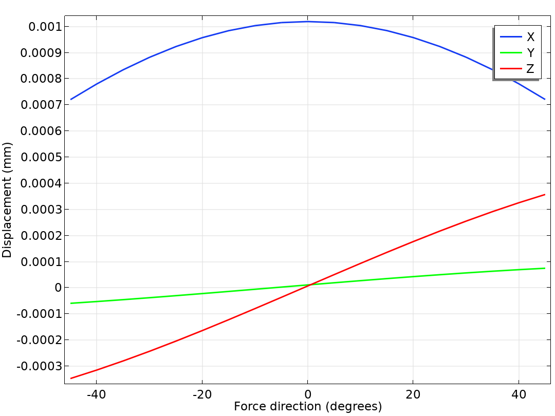
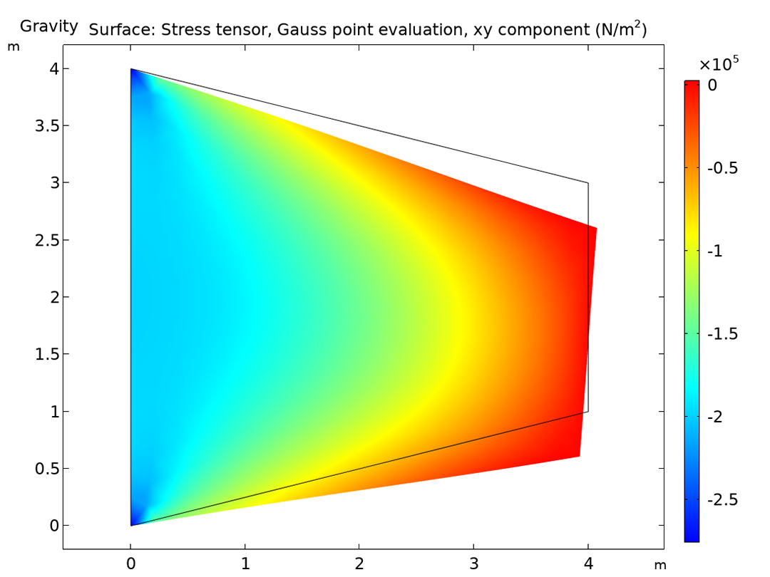
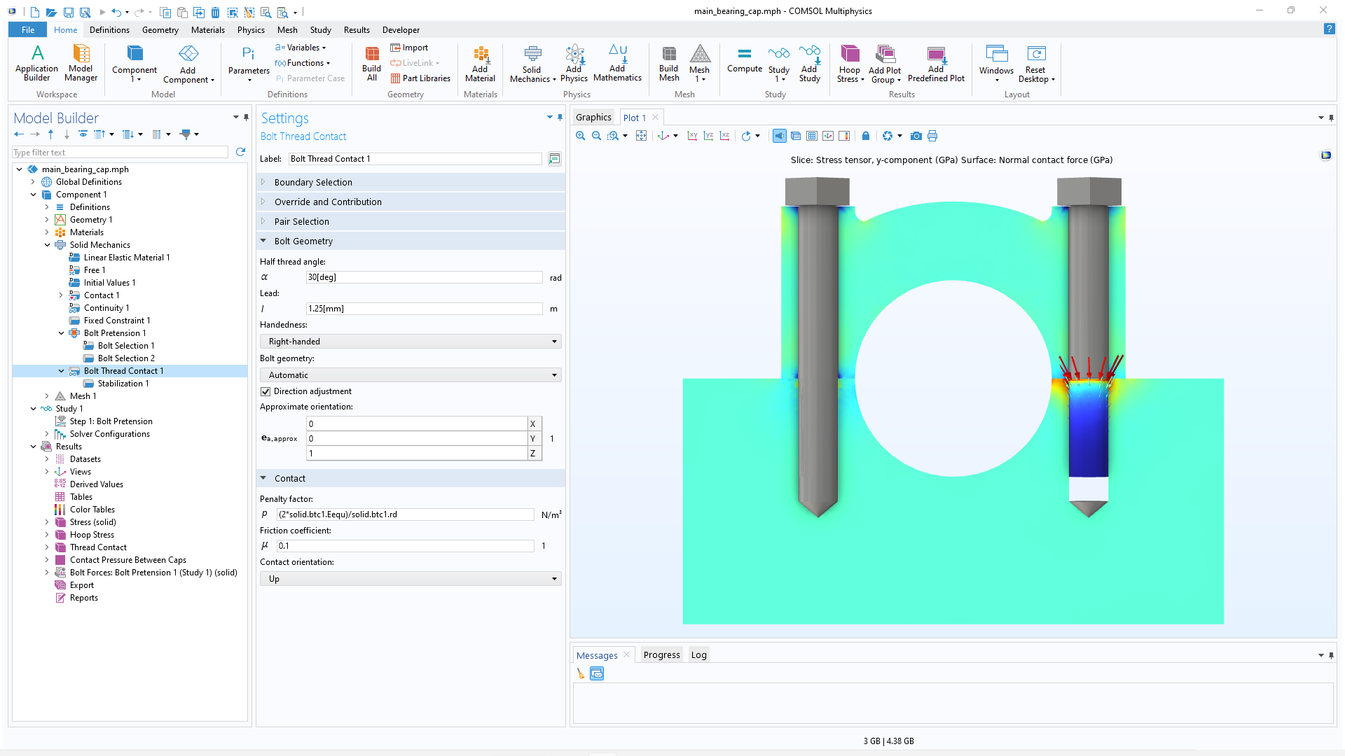
Parametric Analysis
Compute a model with multiple input parameters to compare results.
Run Mechanical Analyses with Extensive Multiphysics Capabilities
The Structural Mechanics Module, an add-on to the COMSOL Multiphysics® platform, is an FEA software package specialized for analyzing the mechanical behavior of solid structures. The module includes features and functionality for solid mechanics and materials modeling as well as the modeling of dynamics and vibrations, shells, beams, contact, fractures, and more. Application areas include mechanical engineering, civil engineering, geomechanics, biomechanics, and MEMS devices.
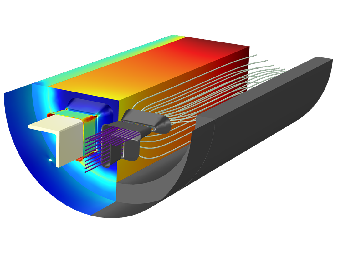
The Structural Mechanics Module offers built-in multiphysics couplings for modeling thermal stress, fluid–structure interaction, and piezoelectricity. Combining its functionality with other modules from the COMSOL product suite allows for advanced simulations involving heat transfer, fluid flow, acoustic, and electromagnetics effects and enables specialized material modeling and CAD import functionality.
Contact COMSOL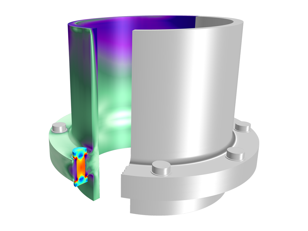
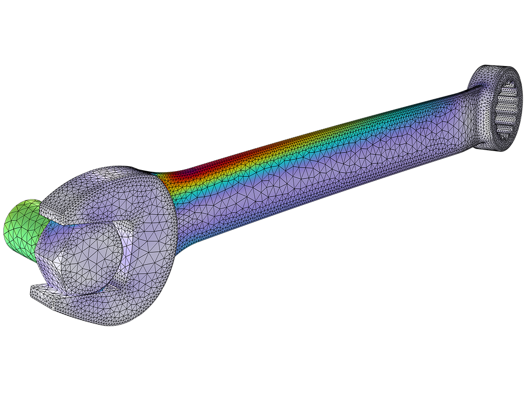
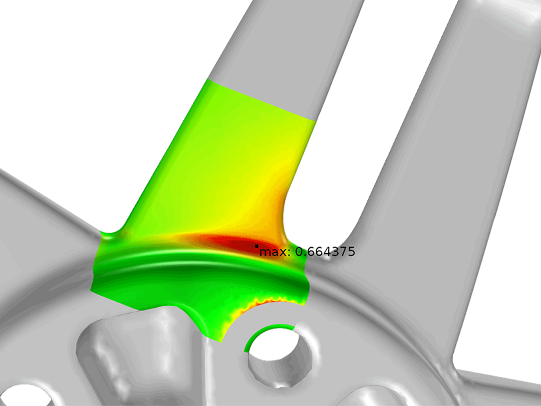
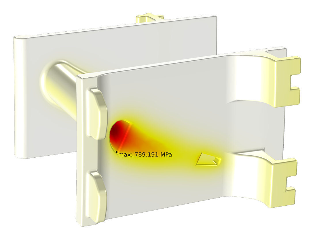
Several analysis types are available for predicting structural performance in a virtual environment. The Structural Mechanics Module can be used to answer questions concerning stress and strain levels; deformations, stiffness, and compliance; natural frequencies; response to dynamic loads; and buckling instability, to name a few.
Compute a model with multiple input parameters to compare results.
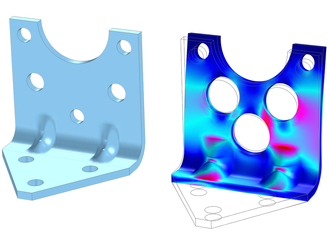
Optimize geometric dimensions, shape, topology, and other quantities with the Optimization Module.
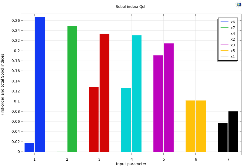
Understand the impact of model sensitivity, uncertainty, and reliability with the Uncertainty Quantification Module.

The Structural Mechanics Module provides a full suite of modeling tools for various types of structural analyses. Based on the finite element method (FEM), its functionality can be used not only for modeling 3D solids, but also in 2D formulations (to simulate plane stress, plane strain, generalized plane strain, and axial symmetry). The module also provides functionality for modeling shells and plates, membranes, beams, pipes, trusses, and wires and for transitioning between different formulations.
There are many options available in the software for the finite element shapes and orders: Triangle, quadrilateral, tetrahedron, hexahedron, prism, and pyramid elements are all available, and users can choose from first-, second-, and higher-order elements, as well as mixed-order elements for multiphysics analysis.
The Structural Mechanics Module provides specialized features and functionality for running a variety of structural analyses and works seamlessly in the COMSOL Multiphysics® platform for a consistent model-building workflow.
The Solid Mechanics interface can be used for modeling in full 3D, 2D (for plane stress, plane strain, and generalized plane strain), 2D axial symmetry, 1D (for plane stress or plane strain in transverse directions), and 1D axial symmetry. The interface provides the most general approach to analyzing solid structures, with built-in multiphysics couplings. Its wide variety of material models makes it possible to accurately describe solid mechanics problems, and it is easy to extend these features via equation-based modeling. Users can define material properties with constant, spatially varying, anisotropic, or nonlinear expressions; lookup tables; or combinations of these. Elements can be activated and deactivated based on user-defined expressions. It is also possible to assign material models to internal or external surfaces. This functionality can be used to model, for example, glue layers, gaskets, fracture zones, or claddings.
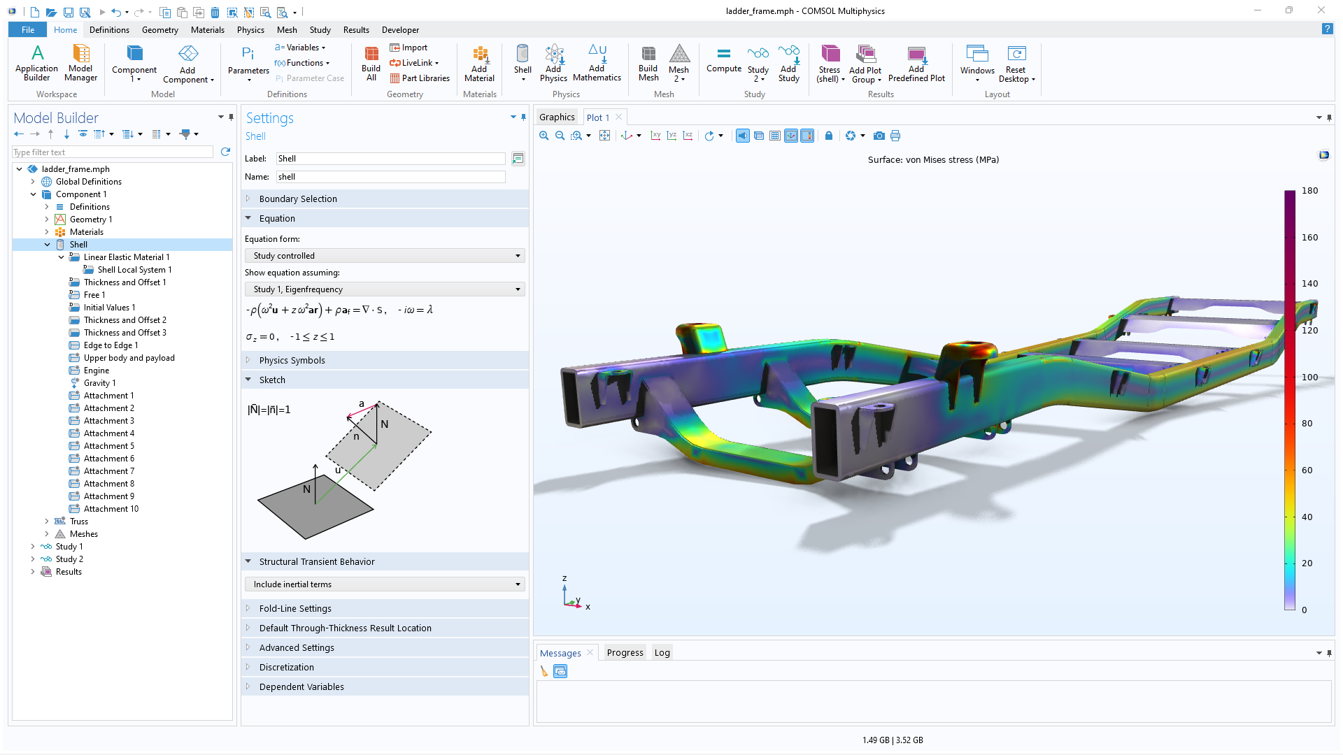
For thin structures, using shell (in 3D and 2D axisymmetry) and plate (in 2D) elements can be very efficient. The formulations allow for the transverse shear deformations needed to model thick shells. It is also possible to prescribe an offset in the direction normal to a selected surface, which simplifies modeling projects involving a full 3D representation of the geometry. The results from a shell element analysis can be visualized using a solid representation.
Very thin structures, such as thin films and fabric, require a formulation with no bending stiffness. This is possible in the Membrane interface, in which curved plane stress elements in 3D or 2D axisymmetry are used to compute in-plane and out-of-plane displacements, including the effects of wrinkling. When studying this type of structure, the ability to start from a prestressed state is used extensively. For membranes that are not prestressed, automatic stabilization is available.
With the Nonlinear Structural Materials Module, a variety of nonlinear material models can be applied to internal and external thin layers. This enables accurate representation of interface layers such as adhesives, gaskets, and claddings, using modeling assumptions that range from full 3D behavior to purely in-plane strain formulations.
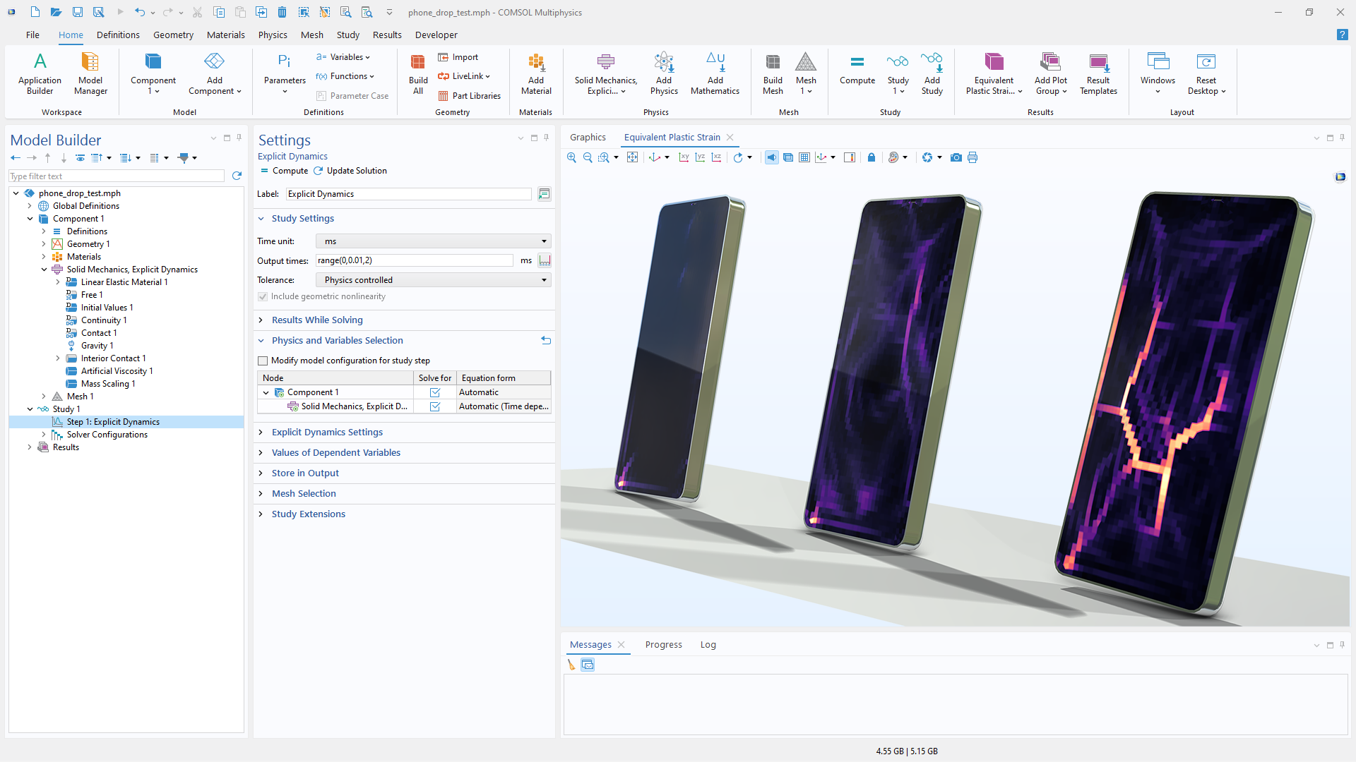
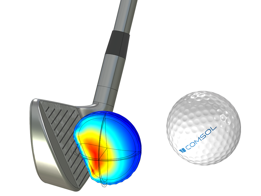
Functionality specialized for time-explicit dynamic analysis enables efficient simulation of fast, transient, and highly nonlinear events such as impacts, wave propagation, and metal forming. The interfaces Solid Mechanics, Explicit Dynamics and Truss, Explicit Dynamics use explicit time integration optimized for large deformations, high strain rates, and general contact conditions. The formulation supports many of the nonlinear materials of the Nonlinear Structural Materials Module, including hyperelasticity and plasticity.
The Elastic Waves, Time Explicit interface can be used to compute the transient propagation of linear elastic waves over large domains containing many wavelengths. It uses a higher-order dG (discontinuous Galerkin)-FEM time-explicit method. The interface is multiphysics enabled and can be seamlessly coupled to fluid domains. Application areas range from micromechanical problems to seismic wave propagation.
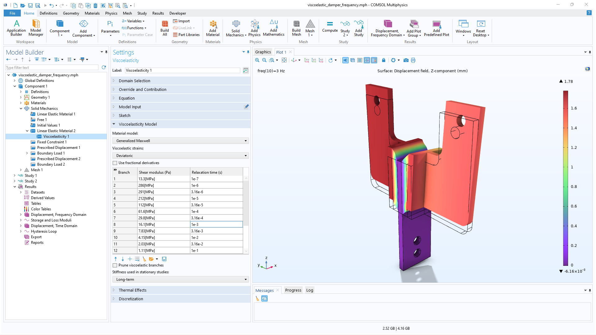
The Structural Mechanics Module provides linear elastic, viscoelastic, and piezoelectric material models, and a wide range of nonlinear material models, including hyperelastic and elastoplastic models, is accessible by adding the Nonlinear Structural Materials Module or the Geomechanics Module.
In addition, there are many capabilities for extending the existing material models or for users to create their own. Expressions that depend on stress, strain, spatial coordinates, time, or fields coming from another physics interface can be entered directly into the input field for a material property. In frequency-domain analyses, complex-valued expressions can be entered. For example, custom differential equations can be added to provide inelastic strain contributions.
The material models can accommodate thermal expansion, hygroscopic swelling, initial stresses and strains, and several types of damping. Material properties can be isotropic, orthotropic, or fully anisotropic. Users can also include their own material models by providing external functions coded in the C programming language.
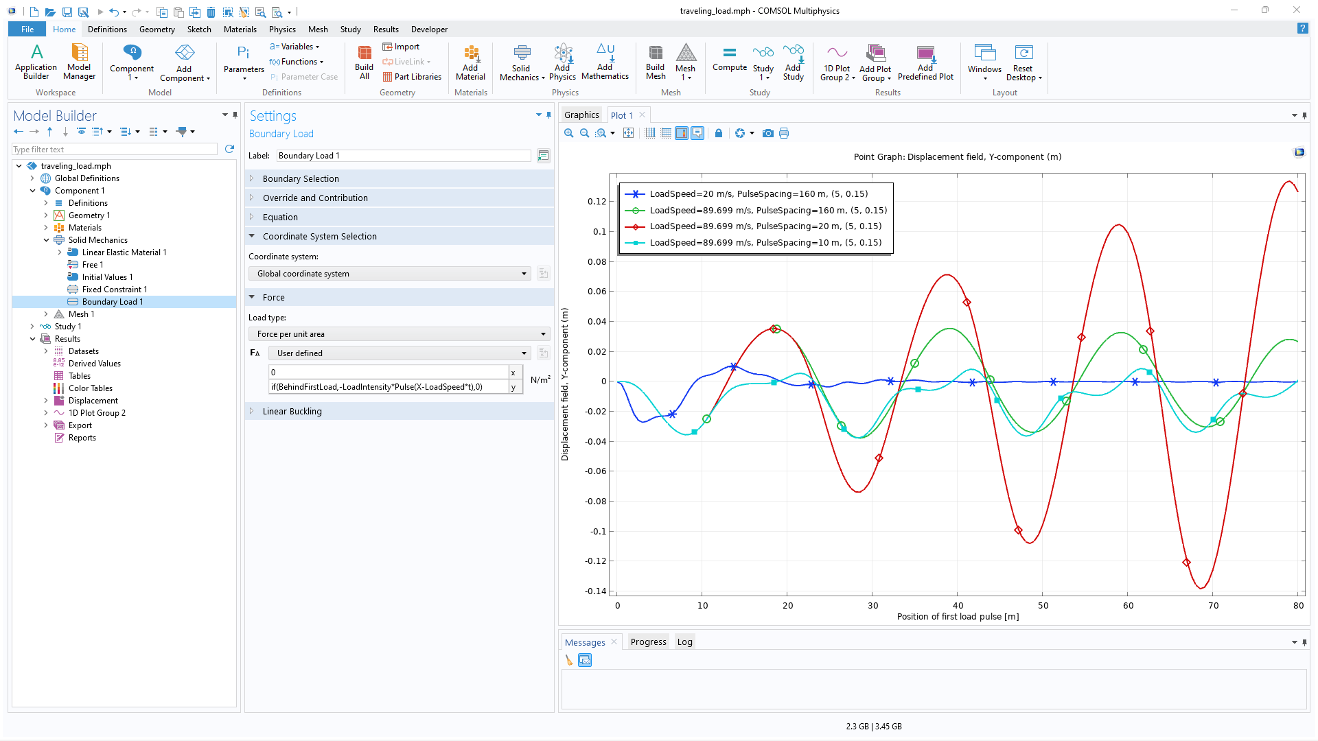
The Structural Mechanics Module offers a multitude of different load and constraint options, which facilitates high-fidelity modeling. There are capabilities for defining distributed loads on domains, boundaries, and edges, follower loads, and moving loads. There is also support for specifying a total force, including gravity or added mass, and including rotating frames with centrifugal, Coriolis, and Euler forces.
For constraining a model, there are springs and dampers, as well as prescribed displacement, velocity, and acceleration. Periodic boundary conditions, low-reflecting boundaries, perfectly matched layers (PMLs), and infinite elements aid in reducing model size for efficient modeling.
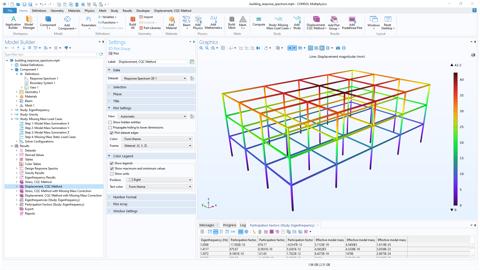
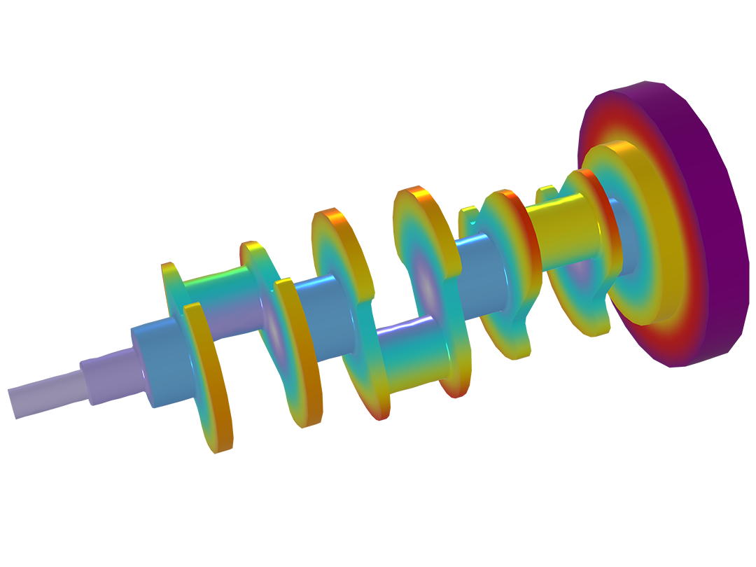
The Structural Mechanics Module covers transient as well as frequency-response analysis. Frequency-response analysis includes eigenfrequency, damped eigenfrequency, and frequency sweep analyses. In addition, specialized study types are available for random vibration and response spectrum analysis. Random vibration analysis allows for inputs based on power spectral density (PSD) as a function of frequency, including uncorrelated as well as fully correlated loads. Response spectrum analysis is used as an efficient method for determining structural response to short, nondeterministic events like earthquakes and shocks.
Component mode synthesis (CMS), also known as dynamic substructuring, reduces linear components to computationally efficient reduced-order models (ROMs) using the Craig–Bampton method. These ROM components can then be used in dynamic or stationary analyses, improving computation time and memory usage.
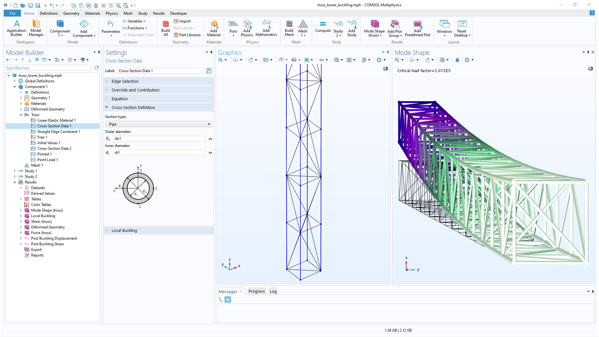
There are specialized element types for modeling beams, described by their cross-section properties. Formulations for both slender beams (Euler–Bernoulli theory) and thick beams (Timoshenko theory) are available. Predefined couplings make it possible to mix beams with other element types to study reinforcements for solid and shell structures. A library of common cross-section types is available as well as functionality for modeling general cross sections.
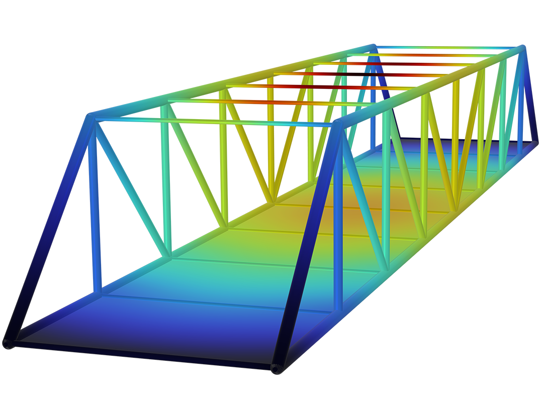
Additionally, the Structural Mechanics Module enables the modeling of slender structures that can only sustain axial forces (trusses and wires). These elements can also be used for modeling reinforcements.
Structural analysis of pipes is similar to that of beams but with the addition of an internal pressure that usually contributes significantly to the stresses in a pipe. Also, in this type of analysis, temperature gradients usually occur through the pipe wall rather than across the entire section. The loads from internal pressure and drag forces can be taken directly from the results of a pipe flow and thermal analysis using the Pipe Flow Module.
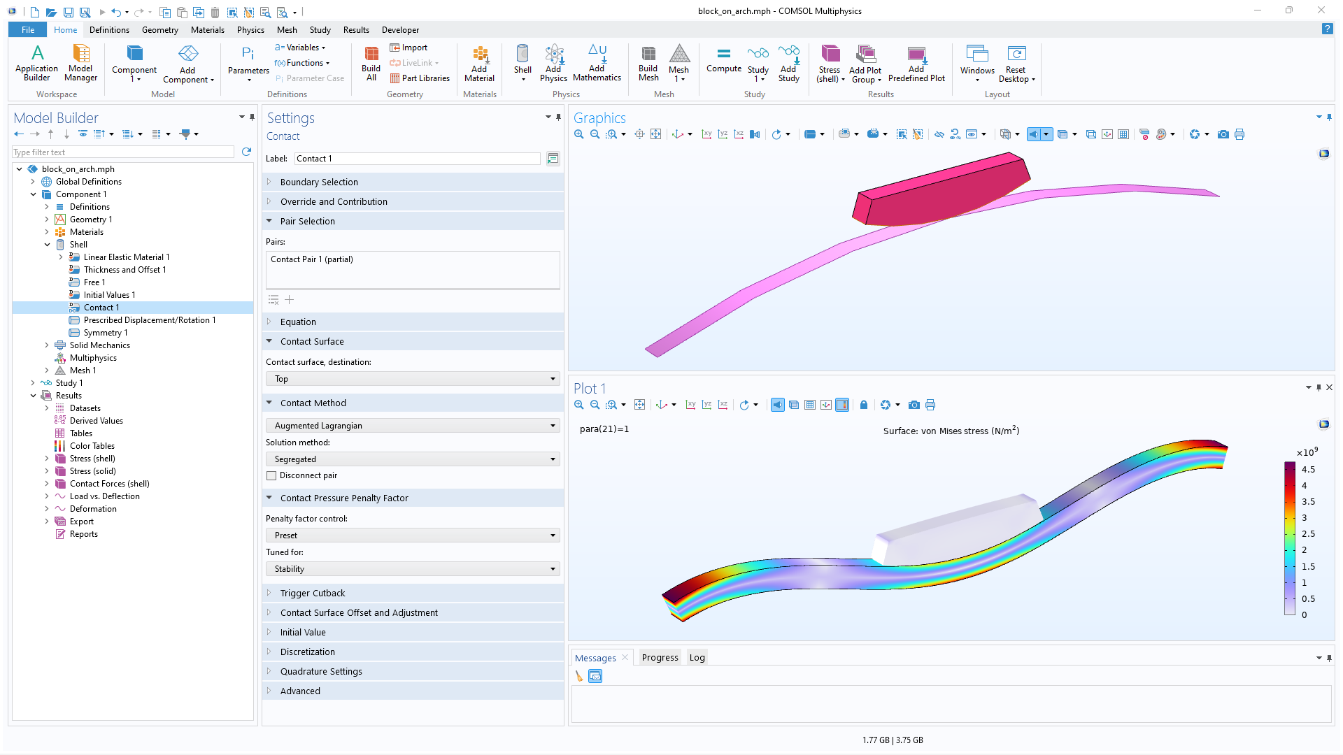
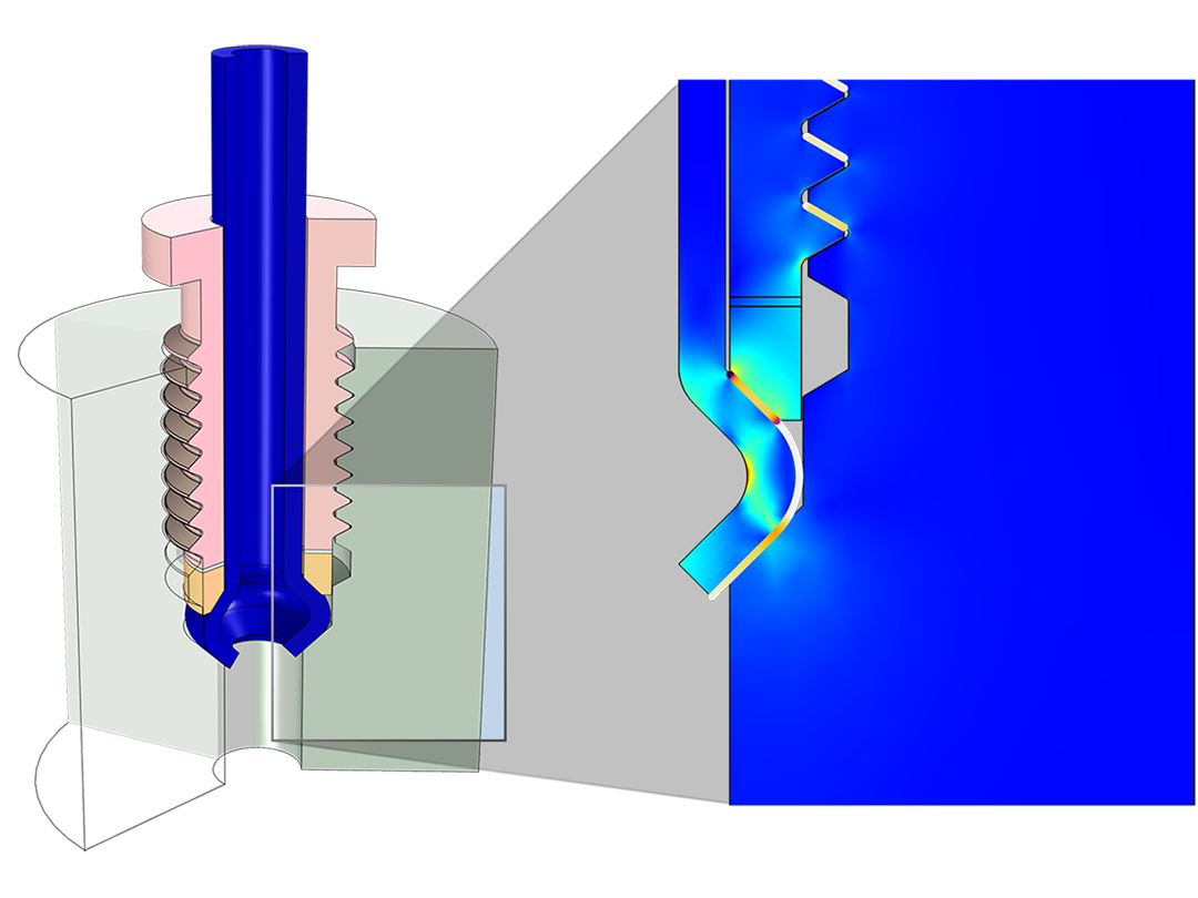
Situations where objects come into contact with each other occur frequently in mechanical simulations. Static and dynamic analyses can include contact modeling, and the objects in contact can have arbitrarily large relative displacements. Additionally, the effects of friction, both sticking and sliding, can be modeled.
The contact analysis functionality also includes capabilities for prescribing adhesion and decohesion between objects in contact and modeling removal of material by wear when objects are sliding relative to each other.
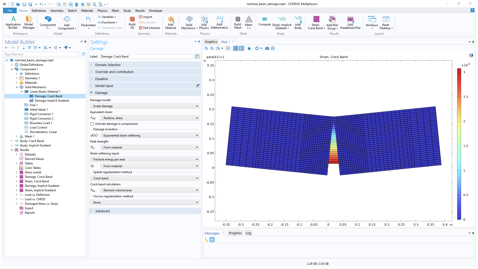
Several different approaches for crack modeling are supported. A crack can either be infinitely thin and represented by a single boundary or represented by disjoint surfaces in the geometry. A crack can have any number of branches and corresponding crack fronts. Effects of crack closure, as well as loads on the crack faces, can be included. Stress intensity factors and energy release rates can be computed in 2D and 3D using J-integral or virtual crack extension methods.
By adding the Nonlinear Structural Materials Module or the Geomechanics Module, users can model damage and cracking in brittle materials according to various criteria.
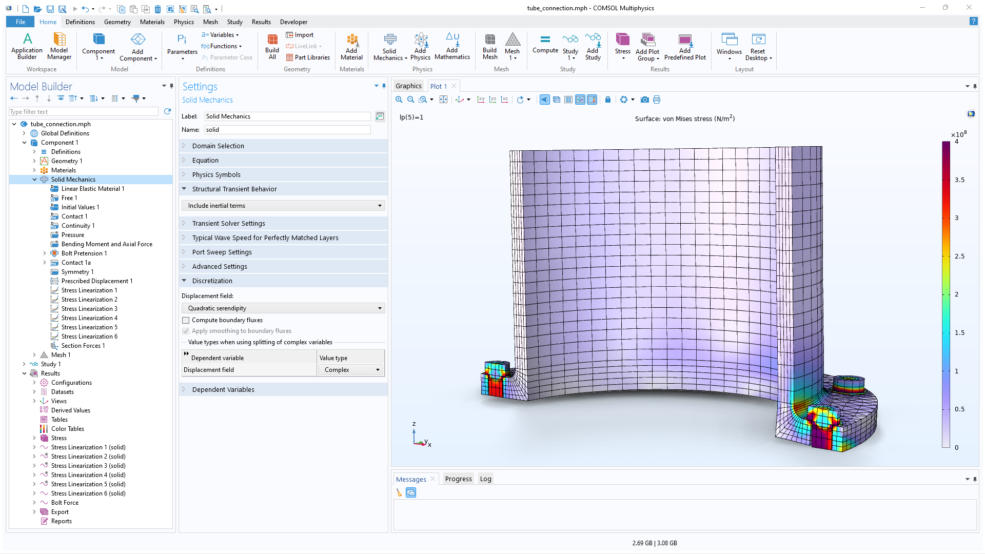
The Structural Mechanics Module includes several structural engineering features that enable users to create real-world models more quickly. These features include boundary conditions such as rigid connectors for modeling rigid bodies and kinematic constraints, bolts with pretension, and stress linearization for analysis of pressure vessels, as well as:
For specialized analyses, completely integrated with the COMSOL Multiphysics® software environment.
The Nonlinear Structural Materials Module and the Geomechanics Module extend the functionality of the Structural Mechanics Module with more than 100 different nonlinear material models.
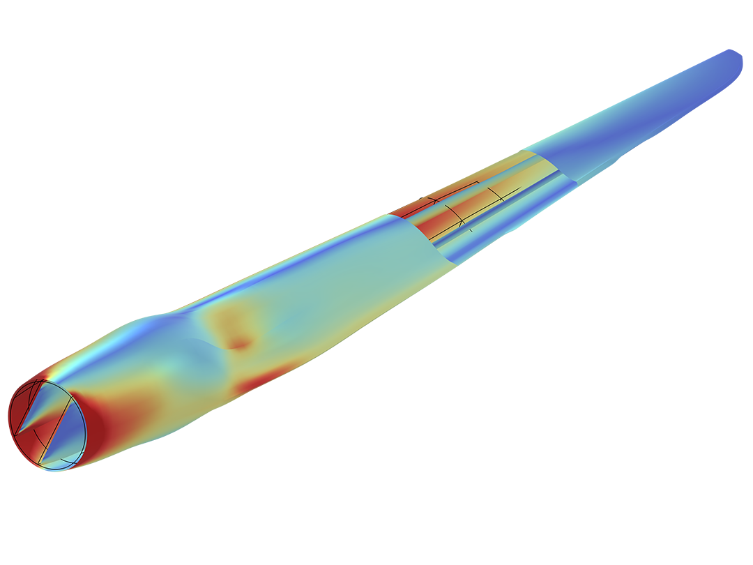
The Composite Materials Module can be added to analyze thin, layered structures (composite materials), such as fiber-reinforced plastic, laminated plates, and sandwich panels found in aircraft components, wind turbine blades, automobile components, and more.
The Fatigue Module can be added to compute the fatigue life of structures. It provides functionality for high-cycle and low-cycle fatigue analyses, harmonic and random vibration fatigue analyses, as well as methods based on rainflow cycle counting.
The Rotordynamics Module can be added to model rotating machines where asymmetries can lead to instabilities and damaging resonances. Users can build rotor components with disks, bearings, and foundations and analyze the results with Campbell diagrams, orbits, waterfall plots, and whirl plots.
Interfacing products to seamlessly connect with COMSOL Multiphysics®.
Geometries in a variety of industry-standard CAD formats can be imported into COMSOL Multiphysics® for simulation analysis using the CAD Import Module. Its available features include automatic repair and cleanup of CAD geometry to prepare it for meshing and analysis, as well as defeaturing tools.
The Design Module also includes these features. Additionally, it supports advanced solid operations for eliminating gaps and intersections when combining components imported from CAD assemblies and 3D CAD operations for editing and creating geometry.
A line of interfacing products, known as LiveLink™ products, can be used to synchronized CAD-native models for use in the COMSOL® software. In addition, geometry parameters can be simultaneously updated in both the CAD program and COMSOL Multiphysics®, and parametric sweeps and optimization can be performed over several different modeling parameters.
Easily combine two or more physics interactions, all within the same software environment.
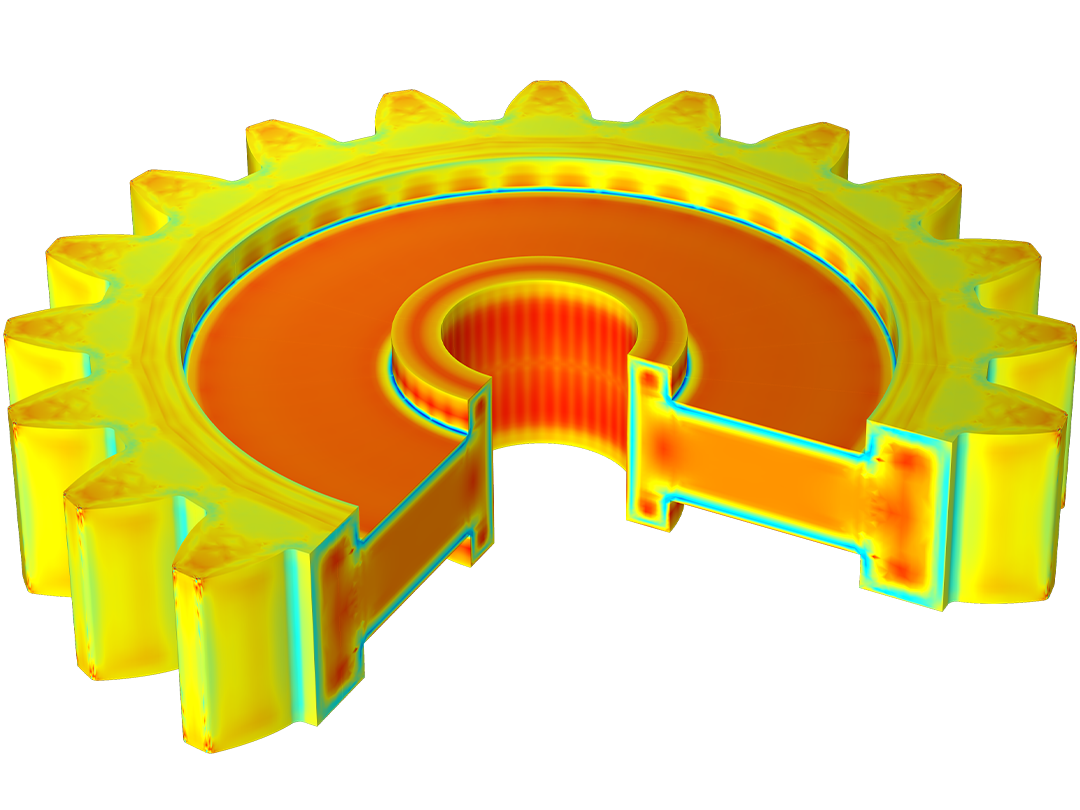
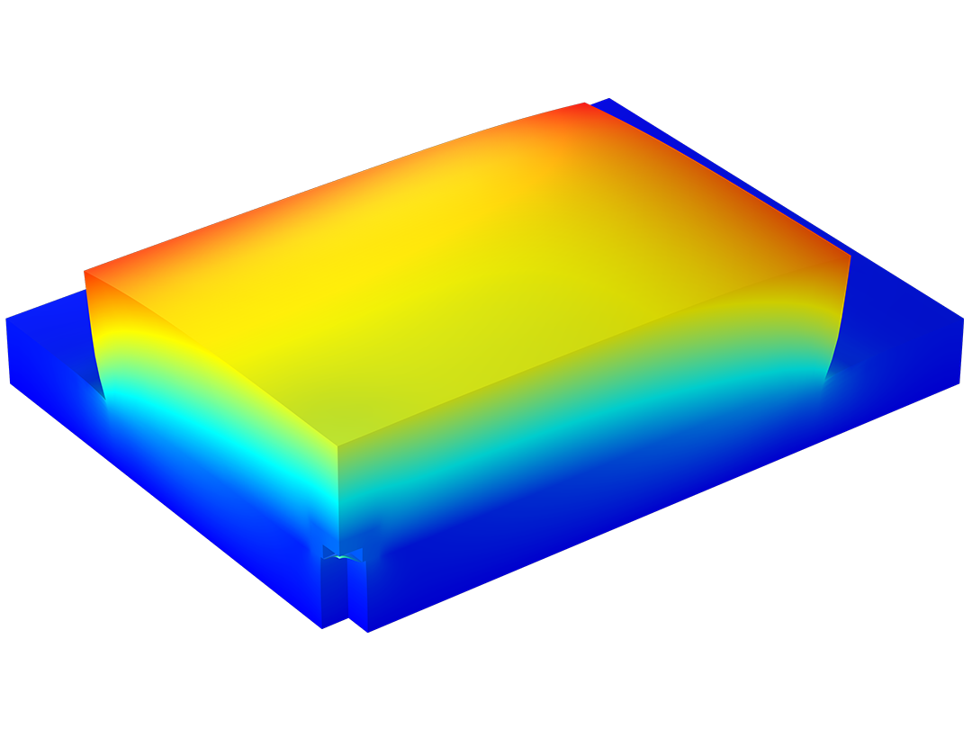
Thermal stress and expansion, with a given or computed temperature field, in solids, shells, and pipes.
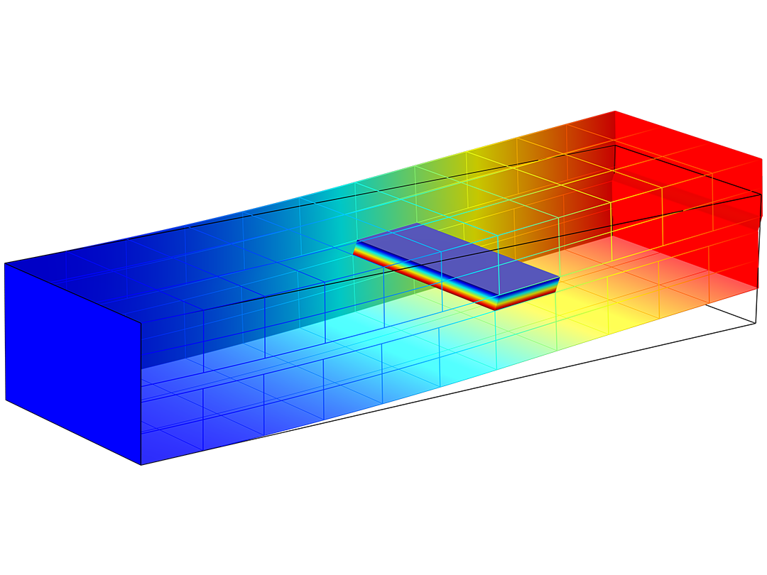
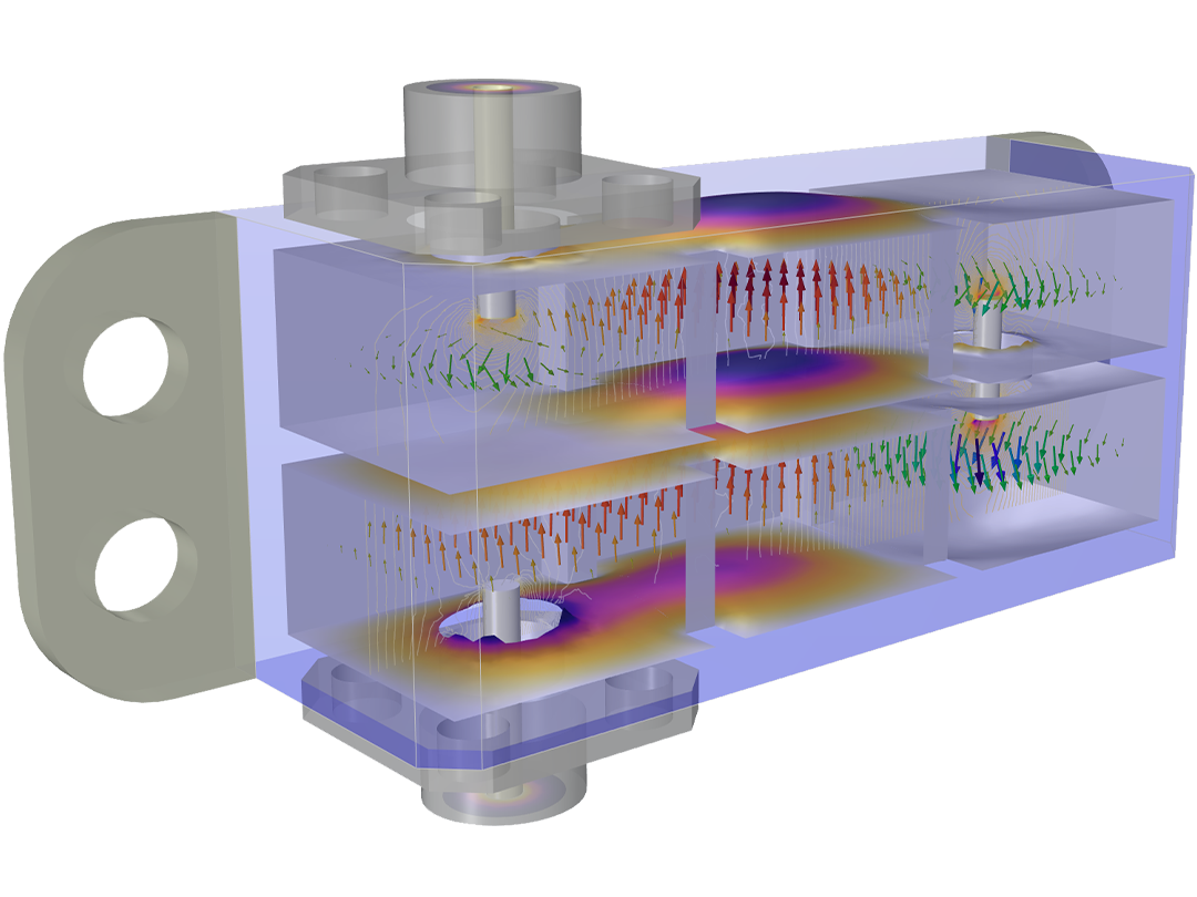
One-way or two-way couplings between a fluid and solid structure, including both fluid pressure and viscous forces.
Stresses and strains of phase-composition-dependent materials during steel quenching and other heat treatment processes.
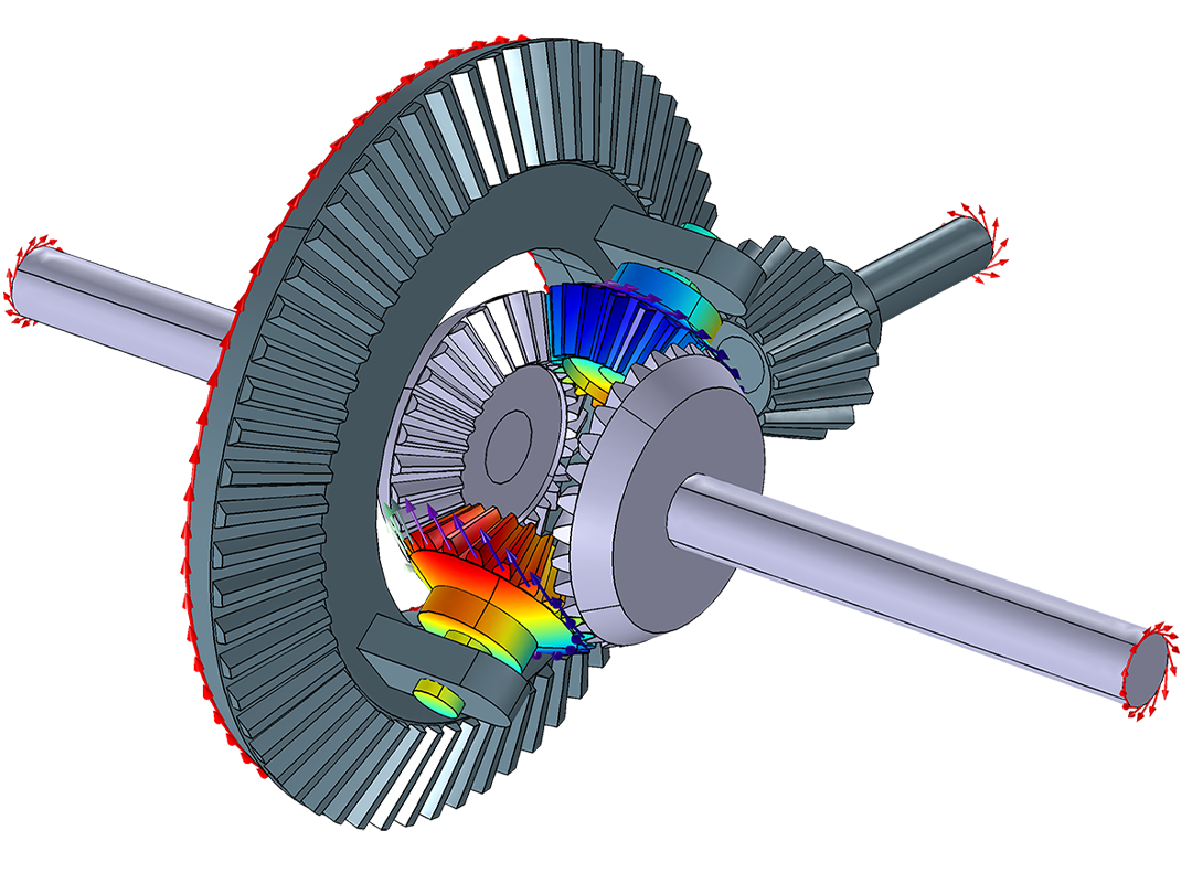
An extensive set of tools for simulating mixed systems of flexible and rigid bodies.
Piezoelectric devices including metallic and dielectric components.
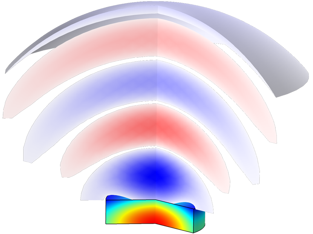
Solid–acoustic, acoustic–shell, and piezo–acoustic interactions, as well as vibration and elastic wave propagation.

Porous media flow coupled with solid mechanics to model poroelastic effects.
Absorption of moisture and hygroscopic swelling in polymers and batteries.

Piezoresistivity, electromechanical deflection due to electrostatic forces, and electrostriction.
Magnetostrictive, electrostrictive, and ferroelectric elastic devices.

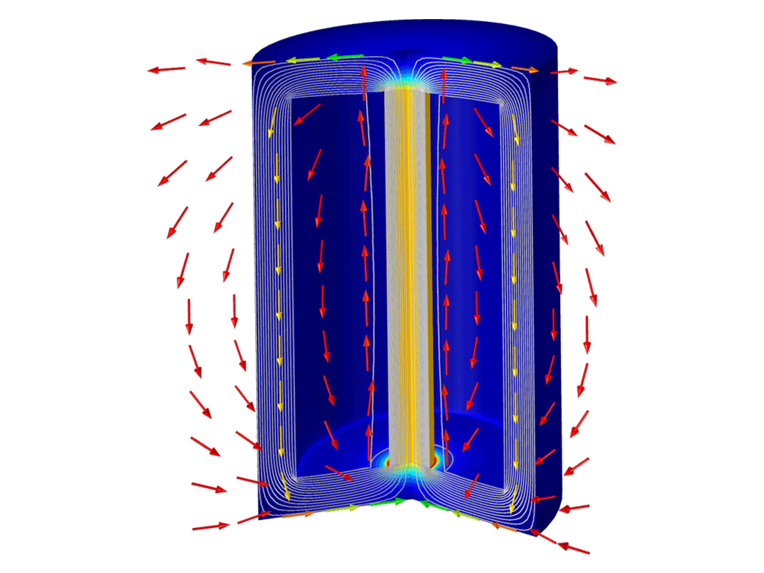
Deformations in electronic devices and electric motors due to electromagnetic forces.
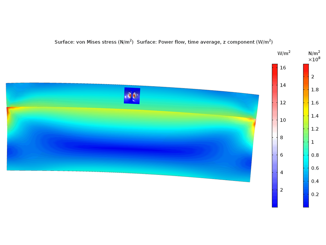
Mechanical deformation and stress affecting the performance of RF and microwave devices and components such as filters.
Stress-induced birefringence in waveguides.

Structural-thermal-optical performance (STOP) analysis on optical systems.
Every business and every simulation need is different.
In order to fully evaluate whether or not the COMSOL Multiphysics® software will meet your requirements, you need to contact us. By talking to one of our sales representatives, you will get personalized recommendations and fully documented examples to help you get the most out of your evaluation and guide you to choose the best license option to suit your needs.
Just click on the "Contact COMSOL" button, fill in your contact details and any specific comments or questions, and submit. You will receive a response from a sales representative within one business day.
Request a Software Demonstration