Modeling the Acoustics of the Liberty Bell in COMSOL Multiphysics^®

This year marks the 250^th anniversary of the U.S. Declaration of Independence, and the Liberty Bell — a symbol of freedom, famous for its distinctive crack — offers a historically significant and physically interesting case study for simulation. In this blog post, I will use the COMSOL Multiphysics^® software to analyze several fascinating aspects of the Liberty Bell, including the structural modes of the bell (with and without a crack). I will also provide new insights into the material properties using uncertainty quantification and attempt to design a perfectly tuned bell using shape optimization.

The Bell that Inspired the Simulation

While in Philadelphia recently for an Acoustical Society of America meeting, I saw the Liberty Bell display and was reminded of some of its history. At the conference, I was also pleasantly surprised to learn about past (Ref. 1) and ongoing (Ref. 2–3) research regarding structural acoustics of the bell.

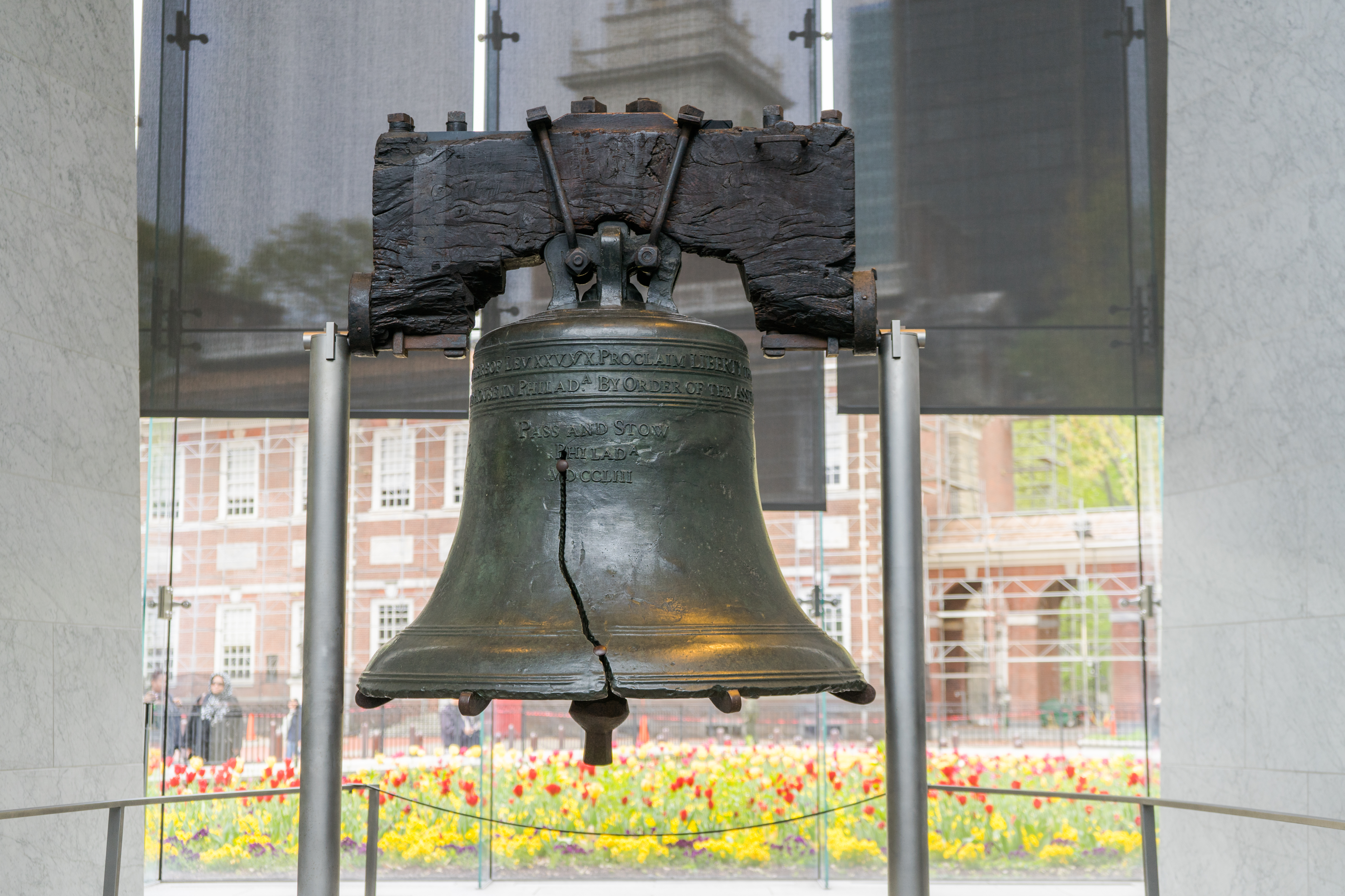The Liberty Bell. Image by William Zhan — Own work. Licensed under CC BY 2.0, via Flickr Creative Commons.

The Liberty Bell was ordered for the Pennsylvania State House and cast by the Whitechapel Bell Foundry in London (Ref. 4). The original imported bell cracked during its first test ring and was recast locally by John Pass and John Stow. The famous crack visible today is a later feature of the recast bell; according to the National Park Service (Ref. 4), its exact origin is not recorded, but a narrow split likely developed in the early 1840s and was widened in 1846 by metal workers to prevent it from spreading further. Today, the Liberty Bell is treasured as a national icon. It is currently on display at the Liberty Bell Center at Independence National Historical Park in Philadelphia, Pennsylvania.

Modeling the Liberty Bell

Our first goal as simulation engineers interested in structural acoustics is to compute the structural modes of the bell. To do this, we will need some baseline material properties, geometry, and physics with boundary conditions. The material properties for so-called bell bronze can vary dramatically, but for now we will assume the elastic modulus, density, and Poisson ratio are constant (E = 120\, \textrm{GPa}, \rho = 8800\,\textrm{kg/m\^{}3}, \nu = 0.34) and employ a linear elastic material model. Since the bells are designed to ring, the structural damping is quite low, so it will be neglected for computing the modes.

The geometry of the bell is very important. In fact, the acoustics of church bells have been analyzed extensively, and bell foundries will typically tune the first five modes with particular ratios in order to achieve optimal tuning. The names of the first five modes as well as the frequency ratios for a well-tuned bell (Ref. 5) are: hum (0.5f_0 ); fundamental, also known as prime, (f_0); tierce (1.2f_0); quint (1.5f_0); and nominal (2.0f_0). It is not known if or how precisely the Liberty Bell was tuned, which is one of the questions the first simulation will investigate.

In order to obtain a realistic geometry, we will utilize a 3D scan of a Liberty Bell replica (see caption). The scan is a surface mesh that contains all the inscriptions, mounting structure, clapper, and some defects from the scan. However, using the geometry tools in COMSOL^®, we extract a representative cross section and revolve this to create the solid geometry. We will also ignore some of the features, since it would add complexity and should not significantly contribute to the ringing modes of the bell.

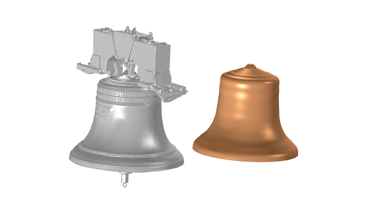At left: Geometry of the Liberty Bell replica from a 3D scan by the VAR Lab at Penn State Behrend, licensed under CC BY 4.0 International. At right: The geometry was modified and defeatured for simulation.

For the physics, we use the Solid Mechanics interface and leave the default Free boundary condition on all boundaries. An eigenfrequency study is used to compute the first five modes of the structure only. The model predicts a fundamental of f_0=336\,\textrm{Hz}. Compared to a perfectly tuned bell, the replica with baseline properties is slightly off tune (see the harmonic ratios below). We should also note that each of these modes has an orthogonal pair (degenerate at the same frequency), which will be important to remember for later analysis.

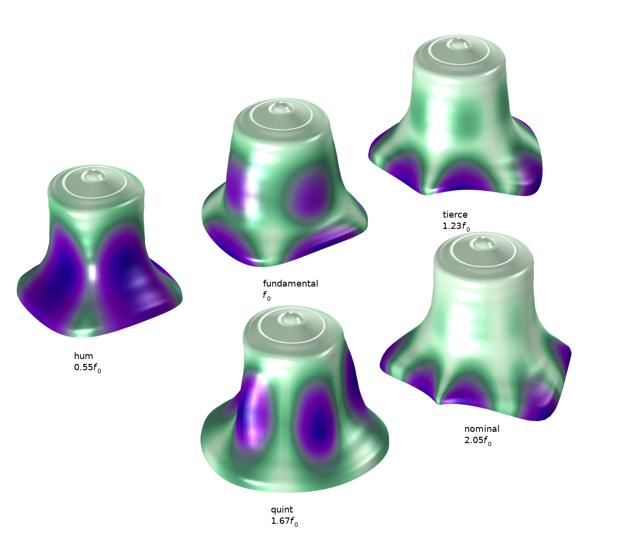First five eigenfrequencies and their corresponding mode shapes.

Uncertainty Quantification

So far, we have computed the modes assuming some baseline properties. The elastic and mass properties of bell bronze, however, are not well documented. Furthermore, its composition could vary depending on the specific alloy mix of the casting. A natural question to ask is: What effect does the uncertainty in the material properties have on the eigenfrequencies? This question can be answered by using the Uncertainty Quantification Module, an add-on to COMSOL Multiphysics^®.

Instead of defining discrete material properties, we will define distribution ranges for them. In particular, we set the properties to be uniformly distributed throughout the following ranges: E = 85-125\, \textrm{GPa}, \rho = 8400-9000\,\textrm{kg/m\^{}3}, \nu = 0.30-0.34. We will use the Uncertainty Propagation study type along with an eigenfrequency reference study to determine a 95% prediction interval for the modes of interest. The method utilizes a surrogate model in order to efficiently compute the uncertainties.

The result from the analysis shows us error bars with the expected range of eigenfrequencies. From these results, we can note that the variation increases with increasing mode number (going from +/- 17 Hz for the hum to +/- 60 Hz for the nominal). Furthermore, experimental measurement from Ref. 1 has modes that do fall within the range of the error bars, giving us confidence that we have reasonably bracketed the properties of the bell.

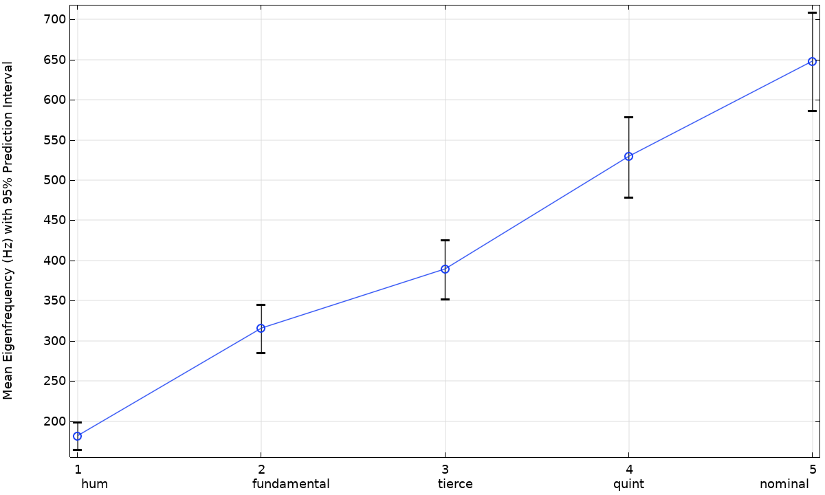The mean eigenfrequencies (blue) and 95% confidence interval (black error bars) for the eigenfrequencies of the bell, given uniform distributions of the mass and elastic material properties.

What About the Crack?

A cracked bell can still vibrate and radiate sound, but the crack can strongly alter its tonal character. To investigate, we add a 1 mm crack to the geometry, qualitatively similar to the location of the large crack. The crack locally reduces stiffness and breaks the axisymmetry of the structure, leading to mode splitting. The formerly degenerate mode pairs split, producing 10 distinct eigenfrequencies over the frequency range considered (shown below at right). This, of course, results in modes that are vastly different from the design guidelines and lack harmony.

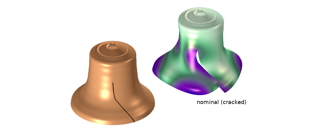
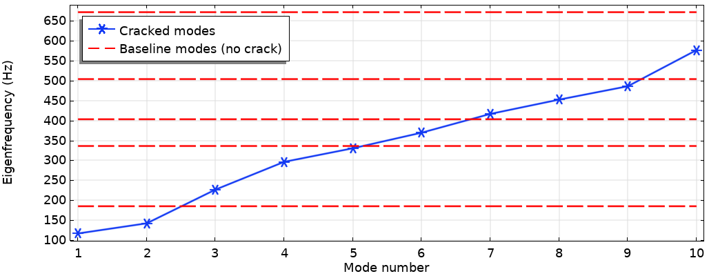
Cracked modes of the structure: cracked geometry and nominal (left) and all computed modes of the cracked bell and baseline bell (right).

Tuning the Bell

Can simulation be used to create a nearly perfect bell? We can set up a shape optimization problem to help find out. The boundaries of the bell are allowed to freely deform in an attempt to minimize the objective function — the squared difference between the current eigenfrequencies and the target ones. The shape optimization runs for 20 iterations, and the result is a new design that achieves the target frequencies within less than 0.02% error for all frequencies! Essentially, it is able to almost perfectly match the guidelines in Ref. 5. Interestingly enough, the new shape closely resembles the baseline shape, which truly provides appreciation for the high precision involved in casting and machining bells for high acoustic quality.

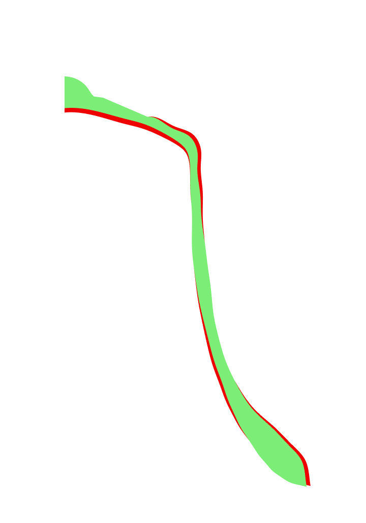
Result of the shape optimization: one half of an axisymmetric view of the bell cross section showing baseline geometry (red) and shape-optimized geometry (green).

Acoustic–Structure Interaction

Lastly, we model the sound radiation response from the defeatured Liberty Bell replica by using the Acoustic–Solid Interaction, Frequency Domain interface. We also assume a loss factor of \eta = 0.001. A boundary load condition is applied on a representative area of where the clapper would strike. The model computes the full field displacements, stresses, and strains, as well as acoustic pressure and sound pressure level (SPL) resulting from the force.

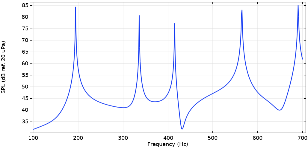SPL vs. frequency for observer location adjacent to the bell at (0,0,-2m).

The results can be animated over an acoustic cycle to get the full picture of the vibroacoustics.

Further Resources

In this blog post, we have presented several structural acoustic simulations of the Liberty Bell. However, the possibilities do not have to end there. Simulation can be used to investigate many other aspects of the bell, including: sound propagation from the Liberty Bell and how far away the bell could be heard, dynamic crack propagation caused by repeated impacts, and molten metal solidification during the bell casting process.

Additional information on the technical topics mentioned in this blog post can be found below:

• Performing Optimization in COMSOL Multiphysics
• Introduction to Uncertainty Quantification
• Getting Started with Modeling Structural Mechanics
• Introduction to Modeling Acoustic-Structure Interactions

References

1. G.H. Koopmann et al., “Tuning a Replica of the Liberty Bell via Material Tailoring: An Application of a Method for Optimal Acoustic Design.” ASME International Mechanical Engineering Congress and Exposition, vol. 35517, American Society of Mechanical Engineers, 2001.
2. J. Young, S. Collier, A. Stearns, and E. Brown, “Modes of America: Computational Acoustics and the Sound of the Liberty Bell,” Presented at the 190th Meeting of the Acoustical Society of America (ASA), Philadelphia, PA, 2026.
3. S. Collier, J. Young, A. Stearns, and E. Brown, “Modal Analysis of a Liberty Bell Replica,” Presented at the 190th Meeting of the Acoustical Society of America (ASA), Philadelphia, PA, 2026.
4. “The Liberty Bell,” June 2025; https://www.nps.gov/inde/learn/historyculture/stories-libertybell.htm.
5. Thomas D. Rossing and Robert Perrin, “Vibrations of Bells,” Applied Acoustics, vol. 20.1, pp. 41–70, 1987.