

The Magnetic Field Formulation interface in the AC/DC Module, an add-on to the COMSOL Multiphysics® software, is useful for modeling materials with nonlinear constitutive relationships. Such materials typically need to be explicitly represented as domains, but sometimes we want to consider very thin conductors. In these situations, it can be advantageous to model the conductor as a boundary condition. It’s quite straightforward to augment the existing interface with additional equations to achieve this. Let’s learn more!
Understanding Thin Conductors
The term thin conductor requires a precise meaning in the current context. We begin with the thickness of the material: It must be small compared to the other dimensions. A PCB trace or conductive tape is a typical example. The material must also be sufficiently thin that the tangential current density can be approximated as uniform through the thickness. This approximation is appropriate when the thickness is much smaller than both the radius of curvature and the skin depth. The latter can be estimated from the material resistivity and characteristic operating frequency. We further assume that conduction currents dominate over displacement currents and therefore neglect displacement-current contributions. Finally, we assume that the magnetic response of the conductor can be neglected, so no magnetic material model is needed.
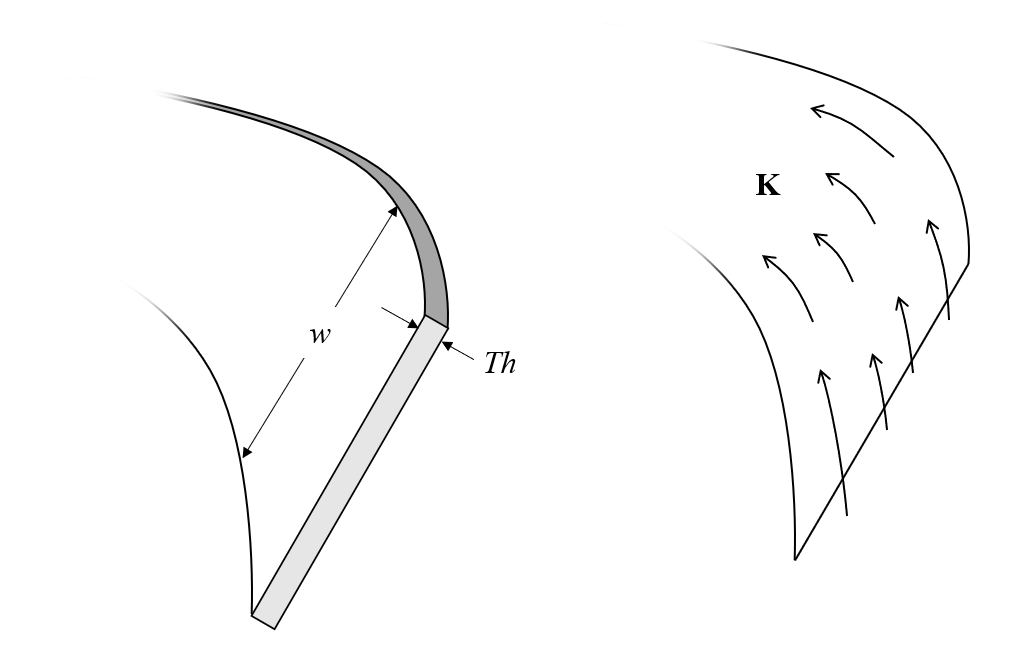
A thin conductor can be modeled as a sheet current.
With the term thin conductor so defined, we can move on to addressing how such a conductor can be modeled. Starting with Maxwell’s equations, we can derive the magnetic field formulation, which uses the finite element method to solve for Faraday’s law within domains:
where the electric field is computed from:
and where the material resistivity, \rho, is the inverse of conductivity and can depend nonlinearly on the magnetic field, the current, or both. Solving these equations also requires a set of boundary conditions and excitations, several of which are addressed in our blog post Modeling of Excitations with the Magnetic Field Formulation.
In addition, in the absence of a surface current, the tangential component of the magnetic field is continuous across an interior boundary:
where the subscripts refer to the up and down sides of the interior boundary. This condition is implicitly satisfied within the Magnetic Field Formulation interface because the tangential magnetic field is represented using curl-conforming vector elements, which maintain tangential continuity across interior boundaries. That is, by default, the interface has a single unknown at the boundary and thus enforces:
However, if there is a nonzero current flowing along a surface, then we have:
This condition is not available within the existing Magnetic Field Formulation interface, but as we are about to see, it’s very easy to add. Along with the current flowing along the surface, we also need the thickness-averaged current density in the conductor and the electric field tangential to the surface:
where Th is the geometric thickness. So, our objective is twofold: Introduce into the existing Magnetic Field Formulation the possibility of a difference in the magnetic field across an interior boundary due to a sheet current and introduce a constitutive relationship of the conductor carrying that current.
Here, we present an intuitive explanation that assumes some familiarity with the finite element method. Since we already have expressions for the tangential current and electric field, we can write the electrical power dissipated over the surface:
In the weak formulation, the corresponding virtual-power contribution is obtained by replacing the surface current with its test variation:
Since the surface current is determined directly from the jump in the magnetic field, its variation is likewise determined by the magnetic-field test functions. This contribution is therefore added to the variational form solved by the finite element method. Several references are provided at the end of this article for readers interested in the details. It’s also worth pointing out that AI tools can often provide specific step-by-step derivations of these types of equations.
Implementation Within COMSOL®
The first requirement for implementing a thin conductor is to allow different magnetic fields on the two sides of a zero-thickness interior boundary. This setup is accomplished by adding an Auxiliary Slit feature to the desired boundaries. The feature disconnects the tangential magnetic-field degrees of freedom on the two sides of the boundary, allowing the fields to differ. We therefore need to add an equation relating these degrees of freedom. The fields on the two sides can be accessed using the up() and down() operators.
 Adding an Auxiliary Slit feature to any interior boundaries of an interface.
As soon as this slit is introduced, we can define a set of variables using the equations developed in the section above. The screenshot below shows a sample of such a definition. Note that the normal vector is defined in terms of <nxmesh,nymesh,nzmesh>, which is the normal as evaluated on the discrete finite element mesh — so, for example, the z-component of the surface current is:
nxmesh*(up(Hy)-down(Hy))-nymesh*(up(Hx)-down(Hx))
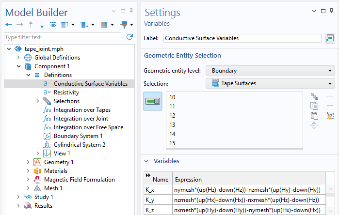 Variables can be defined on the boundaries.
Finally, we need to add a Weak Contribution feature to impose the relationship between the electric field and the surface current. The following contribution is added to the residual:
Es_x*test(K_x)+Es_y*test(K_y)+Es_z*test(K_z)
Keep in mind that the electric field can depend nonlinearly on the surface current via a variable defining the resistivity. For a detailed introduction to weak-form modeling, see this Learning Center series: Modeling with Partial Differential Equations in COMSOL Multiphysics®.
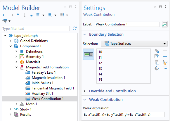 The Weak Contribution feature implements the relationship between the electric field and surface current.
With the Auxiliary Slit and Weak Contribution features added, along with the appropriate variables defined, the implementation is complete. The selected boundaries can now carry surface current, which can also enter or leave adjacent conductive domains. The surface current can be excited using any of the standard approaches for working with the magnetic field formulation discussed in the previously mentioned blog post on magnetic-field excitations.
An Example From the Field of Superconductivity
As an example, we consider an application from the field of superconductivity: two thin superconducting tapes in free space joined by a relatively large metallic conductor, as illustrated below. The superconducting material itself consists of a very thin layer deposited on a relatively insulating substrate. In this example, we assume that currents in the substrate are negligible and therefore omit the substrate entirely. Current can then flow from one superconducting tape, through the metallic joint, and into the other tape.
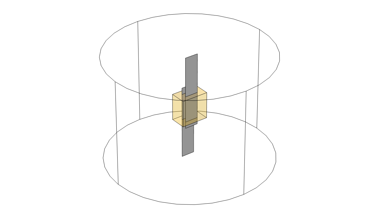 The situation under consideration: Two thin superconducting tapes joined with a metallic joint are modeled within a cylindrical free-space region.
A superconductor has a highly nonlinear relationship between electric field and current density. A commonly used constitutive relationship is the power-law expression for the resistivity:
where E_c is the critical electric field criterion, J_c is the critical current density, and n is the power-law exponent. In general, J_c can depend on magnetic-field magnitude and orientation, as well as on other fields such as temperature; here, we use the simplified form shown above.
A requirement of the magnetic field formulation is that the resistivity can never be exactly zero, so we introduce into the above expression a constant, J_{\min} \ll J_c. This constant is introduced for numerical purposes and is chosen to be sufficiently small so that its effect on the solution is negligible.
Similarly, the resistivity of the surrounding insulating domains cannot be infinite. As a practical starting point, we choose the stabilization resistivity so that the skin depth in these domains is approximately one thousand times the characteristic model length, L_c, to get:
This provides a useful balance between numerical conditioning and artificial dissipation. Nevertheless, the resulting artificial losses should be checked after solving. Because of the large contrast in resistivity and the strongly nonlinear constitutive relationship, the problem is well suited for a direct solver. With a compatible GPU, the solution can also benefit from GPU acceleration.
The excitation is introduced via the Tangential Magnetic Field feature. The prescribed field corresponds to a uniform return current along the exterior of the cylindrical modeling domain. The model is solved in the time domain, with a ramped sinusoidal excitation of current such that the local current density in some parts of the tape periodically exceeds the critical current density. The losses within the thin layer, the metallic domain, and the free-space domain are integrated and compared.
The results below show current flowing along one superconducting tape, through the metallic conductor, and into the other tape. The second plot shows the losses over time and illustrates the effect of the nonlinear constitutive relationship. It also shows that artificial losses associated with the stabilization resistivity are small compared with the conductor losses. It’s also useful to vary the stabilization resistivity and confirm that the losses in the physical conductors remain essentially unchanged. The example also demonstrates an important feature of the formulation: Surface current can naturally enter or leave adjacent volumetric conductors.
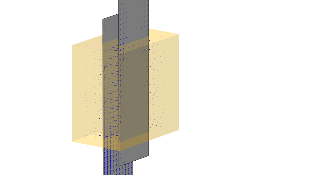 Current flow (blue arrows) along the thin conductive surfaces and through the adjacent volumetric conductor.
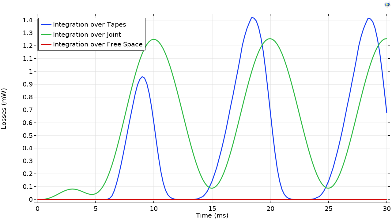 Losses in the thin conductive surfaces, metallic joint, and surrounding free-space domain as a function of time.
Closing Remarks
We have shown how the capabilities of an existing COMSOL Multiphysics® physics interface can be extended by introducing jump conditions and additional equations on interior boundaries. Although the example presented here is from the area of electromagnetic field modeling, this workflow can be useful in other areas of physics.
It’s worth emphasizing that AI tools can be a great help for this kind of model development work. The priming data for most large language models (LLMs) includes the COMSOL documentation and many technical references, so synthesizing this data into a concrete suggestion for a new feature or formulation can be done in only a few minutes.
The formulation developed here enables thin conductors to be modeled as boundaries within the Magnetic Field Formulation interface and is particularly well suited to superconductors with highly nonlinear resistivity. This approach can be applied to other classes of problems, and if you are interested in learning more, please contact us! The model is available via the button below:
References
- J.-M. Jin, Theory and Computation of Electromagnetic Fields, 2nd ed., Wiley-IEEE Press, 2015.
- C. Johnson, Numerical Solution of Partial Differential Equations by the Finite Element Method, Dover, 2009.




Comments (0)