Modeling Ultrafast Heat Transfer with COMSOL Multiphysics^®

Advancements in ultrafast pulsed laser technologies have brought about the need for understanding heat transfer at extremely short time scales. At sub-nanosecond scales, the conventional heat equation breaks down and we must employ more refined models, such as hyperbolic heat transfer equations and two-temperature models. In this blog post, we briefly review the relevant theory for the most common non-Fourier heat transfer models and see how they can be implemented in the COMSOL Multiphysics^® software.

Revisiting the Heat Equation

We begin by briefly recapping one of the most commonly encountered partial differential equations in science and engineering: the heat equation for solids. Our starting point is the energy equation, or the continuity equation for temperature T:

where C=\rho C_p is the volumetric heat capacity, \mathbf{q} is the heat flux, and S is the volume heat source.

This is fundamentally an expression of energy conservation and thus must always hold, regardless of spatial and temporal scale. To get a closed-form PDE for T, we need to find an expression for \mathbf{q}. The simplest and most intuitive choice is Fourier’s law, which states that the heat flux is proportional to the temperature gradient:

The proportionality factor, k, is called the thermal conductivity. Substituting this into the continuity equation yields the familiar heat equation,

This is a parabolic PDE, hence the name parabolic one-step (POS) model. (The meaning of “one-step” will become clear later in this blog post.)

We can gain some insight into the behavior of this equation by considering a semi-infinite (x \geq 0) domain of medium with the surface at x=0 held at temperature T_0, while the initial temperature of the rest of the domain is T_i. This problem has an analytical solution, given by

where \alpha = k/C is the thermal diffusivity of the medium and \mathrm{erf} denotes the error function. And animation of this solution is shown below. From the above expression, it is clear that the effect of the boundary condition at x=0 is felt everywhere immediately, which violates the special theory of relativity. This is a consequence of the rather strong assumption used in deriving this equation; namely, Fourier’s law.

Despite its name, Fourier’s law is really a phenomenological relationship, whose rigorous derivation from first principles involves several approximations. It should be noted, however, that at conventional time- and length scales, the spatial transport of energy is fast enough to be considered instantaneous, so this shortcoming of the heat equation can safely be ignored for most engineering purposes. 

Animation of the time evolution of the solution of the heat equation for a simple semi-infinite domain.

Beyond Fourier’s Law

As we move to shorter time scales, we can no longer assume that the spatial transport of energy is instantaneous, as we did above. Further, we must also account for the finite speed of energy transfer between the electrons and the lattice. Below, we will see how the former leads to hyperbolic heat transfer and the latter to two-temperature models (Ref. 1).

Hyperbolic Heat Transfer

Instead of assuming the heat flux to respond to the temperature gradient instantaneously, we may propose a “laggy” Fourier law as follows:

The lag time \tau should correspond to the electron relaxation time; i.e., the electron mean free time. Provided it is sufficiently small, the above expression can be expanded in a Taylor series, yielding:

This expression is known as the Cattaneo–Vernotte model (Ref. 2). Substituting it into the continuity equation (after differentiating the latter with respect to time) gives the hyperbolic one-step (HOS) model:

This hyperbolic PDE resembles the wave equation, and as we will see below, the finite speed of heat transfer indeed results in the appearance of “thermal waves.”

Two-Temperature Models

Lifting the assumption that the electrons and the lattice are always in local thermal equilibrium requires the introduction of two separate temperature fields (the lattice temperature T_l and the electron temperature T_e) as well as a coupling between them, G. Initially, the energy of the laser is absorbed by the electrons, resulting in a sharp rise in T_e (step 1), which then couples to T_l (step 2). The diffusion of heat through the lattice is negligible compared to its electronic transport at sub-nanosecond time scales, so we end up with the following governing equations:

This is known as the parabolic two-step (PTS) model. We could eliminate T_e to obtain a closed-form PDE for T_l, but this results in cumbersome cross terms. It is more convenient to retain this form of a coupled PDE and domain ODE. An estimate for the electron-lattice coupling parameter G can be obtained by integrating the electron–photon energy exchange rate over all possible transitions (Ref. 3). 

We can additionally account for the finite propagation speed of the electronic thermal energy to obtain the hyperbolic two-step (HTS) model. In analogy with the above model, if we neglect lattice diffusion, the model can be expressed as:

Further Generalizations

There are several additional effects we may need to account for to obtain accurate results, such as:

• Allowing lag time of the temperature in addition to the heat flux, resulting in the dual phase lag (DPL) model
• Including lattice diffusion in the above two-temperature models, leading to the dual parabolic two-step (DPTS) and dual hyperbolic two-step (DHTS) models
• Explicitly modeling carrier dynamics using a two-temperature drift-diffusion type formulation, known as the semiclassical two-step (STS) model
• Accounting for radiative heat transfer

While outside the scope of this blog post, for many applications, it is crucial to account for more complex processes that can take place during ultrafast heating, such as ablation and melting. 

Implementing Non-Fourier Heat Transfer in COMSOL Multiphysics^®

By default, the heat transfer interfaces in COMSOL Multiphysics^® support the POS model only, but implementing hyperbolic heat transfer and two-temperature models in the software with the help of the PDE and ODE interfaces is straightforward.

As a sample problem, we consider a gold film with a thickness of 200 nm irradiated by a laser pulse with absorbed fluence \Phi _p = 1\,\mathrm{J}/\mathrm{m}^2, here assumed independent of the electron and lattice temperature and Gaussian temporal distribution of pulse width t_p = 1 \, \mathrm{ns}, \; 100 \, \mathrm{ps} , \; 100 \, \mathrm{fs}, and 10 \, \mathrm{fs}. \Phi _p contains information about the wavelength of the laser since it depends also on the reflectivity of the film. We also assume the beam radius to be large compared to the penetration depth d of the beam so that the problem becomes one dimensional. Thus, the volume heat source due to the pulse can be written as (Ref. 1):

The prefactors ensure the correct normalization of the total absorbed pulse energy. This pulse is centered at t=0, so we start the simulation at t=-2t_p to capture the full pulse. We adopt the material parameters reported for gold in Ref. 3 and assume them to remain constant.

Hyperbolic Heat Transfer

To include the second-order time derivative of the HOS model, we need to use a General Form PDE interface. The required settings are shown below.

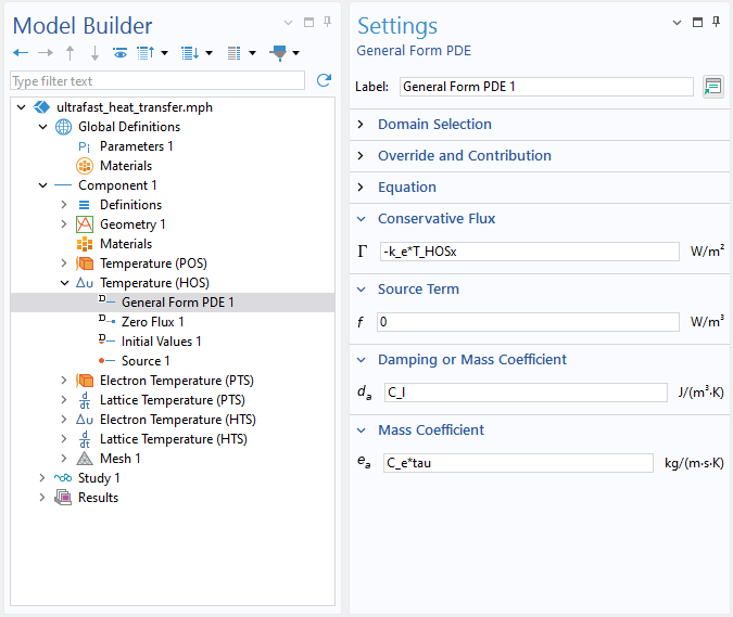Implementation of the HOS model in COMSOL Multiphysics^®. To include the second-order time derivative, we need to use the General Form PDE interface.

Two-Temperature Models

To implement the PTS model, we can model the electron temperature with the predefined Heat Transfer interface, and since the lattice diffusion is ignored in this model, a domain ODE is sufficient to solve for the lattice temperature. The required settings are shown below.

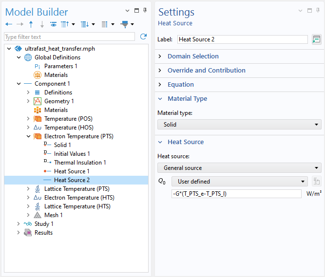
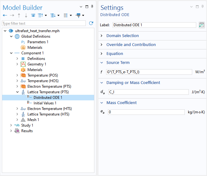
Implementation of the PTS model in COMSOL Multiphysics^®. For the electron temperature (left), we can use the default Heat Transfer interface with an additional source due to the coupling. For the lattice temperature (right), use a Distributed ODE interface with the coupling specified as a source term.

In analogy to the above settings, we can also implement the HTS model by using another General Form PDE interface instead of the Heat Transfer interface for the electron temperature. Note that in this model, the thermal conductivities are considered to be constant scalars, but both the Heat Transfer interface and the General Form PDE interface support coefficients that depend on temperature, for instance, and that are tensorial, for modeling anisotropic heat transfer.

Results and Discussion

Let’s first take a look at the results obtained for t_p = 1 \, \mathrm{ns}. The spatial distributions of the lattice temperatures after irradiation are shown in the figure below. We can see that at this pulse duration, the different formulations give nearly identical results, as expected.

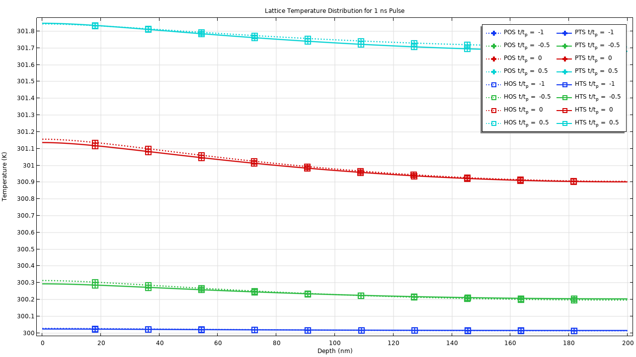Plot of the lattice temperature as a function of depth for a pulse duration of 1 ns. All four models predict nearly identical results at this time scale.

Next, we look at the same plot for t_p = 100 \, \mathrm{ps}, shown in the figure below. A clear discrepancy between the one-step models (POS and HOS) and two-step models (PTS and HTS) emerges: The one-step models predict higher lattice temperature near the irradiated surface due to neglecting the relatively faster electronic heat transfer. However, there is no perceptible difference between the parabolic models (POS and PTS) and hyperbolic models (HOS and HTS) yet.

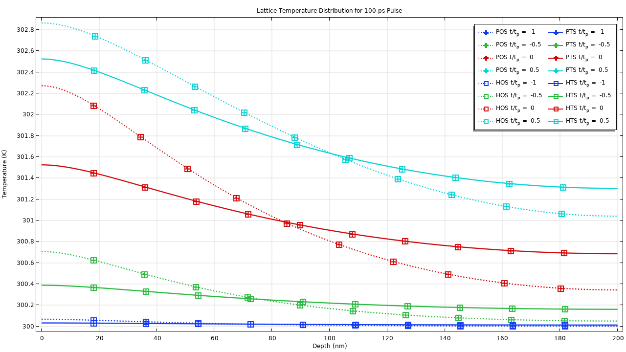Plot of the lattice temperature as a function of depth for a pulse duration of 100 ps. The one-step models (POS and HOS) predict higher lattice temperatures near the irradiated surface.

This discrepancy becomes more pronounced as we move into the femtosecond regime with t_p = 100 \, \mathrm{fs}, as shown in the plot below.

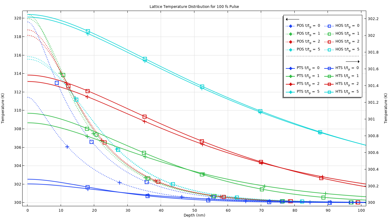Plot of the lattice temperature as a function of depth for a pulse duration of 100 fs. The effect of the second-order time derivative included in the hyperbolic models (HOS and HTS) starts to emerge.

Now the predictions of the one-step models are several hundred degrees higher, and the hyperbolic models exhibit higher temperatures near the irradiated surface than the corresponding parabolic models due to the finite speed of electronic heat transfer.

So far, we have considered only the lattice temperatures. We can get an idea of the difference in the behavior of electron and lattice temperature, by plotting the electron temperature on the same plot, but with a different scale. The result is shown as an animation below.

Animation showing time evolution of the electron (left) and lattice (right) temperature distributions for the 100 fs pulse.

Last, to elucidate the effect of including the second-order time derivative further, let’s compare the electron temperature distribution predicted by the two-step models for t_p = 10 \, \mathrm{fs}. We can now clearly see a thermal wave propagating into the film, which is shown in the figure below. It should be noted that at this pulse length, the electron temperature attains values high enough to warrant inclusion of radiative heat transfer, which is ignored in the present model.

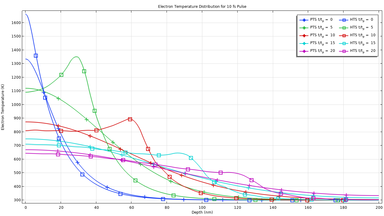Plot of the electron temperature as a function of depth for a pulse duration of 10 fs. We see the propagation of a heat wave predicted by the HTS model.

Finally, to get a sense of the dynamics of the heat transfer through the thin film, we can plot the time dependence of the temperature at the front surface (irradiated surface) and the rear surface. However, due to the large discrepancy in scale, we must normalize each data series by its respective maximum temperature.

The result is shown in the figure below for a pulse duration of 100 fs. At this time scale, the difference between the parabolic and hyperbolic models is moderate, but the one-step models fail to predict the qualitative behavior of the temperature at the rear surface. The one-step models show a monotonically increasing temperature, whereas the two-step models predict that the temperature of the rear surface reaches a maximum due to the electron–lattice relaxation taking place more slowly than the electronic heat transfer. These results agree well with Figs. 3 and 4 of Ref. 3.

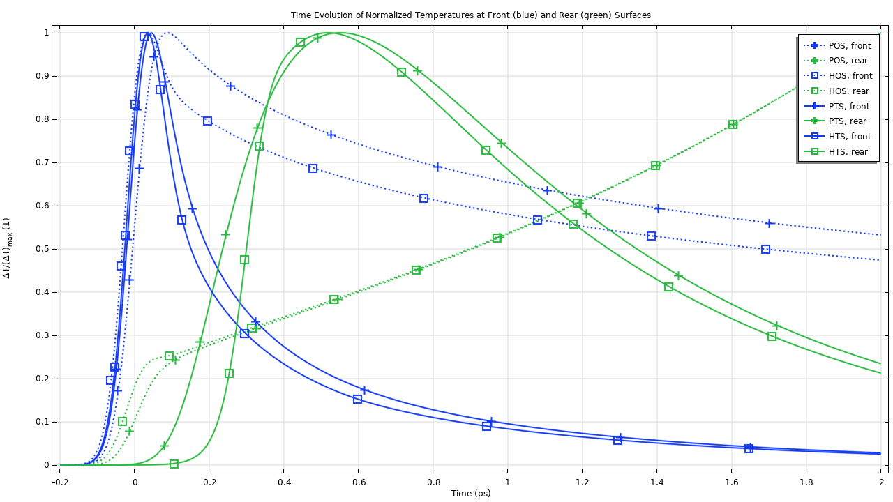Time evolution of the normalized electron temperature (for two-step models) and lattice temperature (for one-step models) for a pulse duration of 100 fs at the front and rear surfaces of the film.

Conclusion

In this blog post, we have seen how COMSOL Multiphysics^® can be used to simulate ultrafast heat transfer processes by implementing four simple and important non-Fourier heat transfer models, namely the parabolic one-step (POS), hyperbolic one-step (HOS), parabolic two-step (PTS), and hyperbolic two-step (HTS) models.

Next Step

Download the model file for the example featured here:

References

1. V.E. Alexopoulou and A.P. Markopoulos, “A Critical Assessment Regarding Two-Temperature Models: An Investigation of the Different Forms of Two-Temperature Models, the Various Ultrashort Pulsed Laser Models and Computational Methods,” Arch Computat Methods Eng, vol. 31, pp. 93–123, 2024. https://doi.org/10.1007/s11831-023-09974-1
2. Y. Zhang, D.Y. Tzou, and J.K. Chen, “Micro- and Nanoscale Heat Transfer in Femtosecond Laser Processing of Metals”, High-Power and Femtosecond Lasers: Properties, Materials and Applications, eds. P.H. Barret and M. Palmerm, Nova Science Publishers, Inc., Hauppauge, NY, ch. 5, pp. 159–206, 2009. https://arxiv.org/abs/1511.03566
3. T.Q. Qiu and C.L. Tien, “Heat Transfer Mechanisms During Short-Pulse Laser Heating of Metals.” ASME J. Heat Transfer, vol. 115, iss. 4, pp. 835–841, 1993. https://doi.org/10.1115/1.2911377