

As discussed previously on the blog, iterative methods efficiently eliminate oscillatory error components while leaving the smooth ones almost untouched (smoothing property). Multigrid methods, in particular, use the smoothing property, nested iteration, and residual correction to optimize convergence. Before putting all of the pieces of this proverbial puzzle together, we need to introduce residual correction and dive a bit deeper into nested iteration. Let’s begin with the latter of these elements.
Nested Iteration
In our earlier blog post, we explained that oscillatory waves of \Omega^{h} appear as smoother waves on the coarser grid \Omega^{2h} (\Omega^{h} has been used to denote the grid with a spacing h). On the same line, we can show that the smooth waves on \Omega^{h} appear more oscillatory on \Omega^{2h}. It is a good idea then to move to a coarser grid when convergence begins to stall. Predominant smooth waves on \Omega^{h} will appear more oscillatory on \Omega^{2h}, where the smoothing property of iterative methods makes them more efficient.
As such, coarse grids can be used to generate improved initial guesses as in the following nested iteration procedure:
- Iterate on Av = f on the coarsest grid
- …
- Iterate on Av = f on \Omega^{4h} to obtain an initial guess for \Omega^{2h}
- Iterate on Av = f on \Omega^{2h} to obtain an initial guess for \Omega^{h}
- Iterate on Av = f on \Omega^{h} to obtain a final approximation to the solution
Nested iteration seems to be a good procedure, but once we are on the fine grid, what happens if we still have smooth error components and convergence begins to stall? The residual equation comes in hand at this point, with multigrid methods showing us how to use it together effectively with nested iteration.
Note: Information between the grids is transferred through two functions: prolongation (from a coarse grid to a fine grid) and restriction (from a fine grid to a coarse grid) operators. Although they represent an important part of multigrid methods and are a fascinating subject, we will not cover them in today’s blog post for the sake of brevity.
The Residual Equation and Coarse Grid Correction
The solution is unknown while we compute the approximate solution and the norm of the algebraic error e = u -v is a measure of how well our iterative method is converging to the solution. (The equation can also be written as u = v + e.) Since the algebraic error is unknown as well, we have to rely on a measurement that can be computed: the residual r = f -Av.
After some algebra, we identify the important relationship between e and r: the residual equation Ae = r. The residual equation is important, as it will lead us to the idea of residual correction. That is, we compute the approximate solution v_0 and r, solve directly thanks to the residual equation, and then compute a new approximate solution v_1 using the definition of the algebraic error: v_1 \leftarrow v_0 + e.
Further, with the residual equation, we can iterate directly on the error and use the residual correction to improve the approximate solution. While iterating on \Omega^{h}, convergence will eventually begin to stall if smooth error components are still present. We can then iterate the residual equation on the coarser grid \Omega^{2h}, return to \Omega^{h}, and correct the approximated solution first obtained here. The procedure, called coarse grid correction, involves the following steps:
- Iterate v_1 times on A^{h}v^{h} = f^{h} to obtain the approximate solution until reaching a desirable convergence
- Compute the residual r^h = f^h -A^{h}v^{h}
- Solve the residual equation A^{2h}e^{2h} = r^{h} to obtain the algebraic error e^{2h} (the restriction operator needed by r^{h} has been omitted)
- Correct v^{h} with e^{2h}:e^{2h}: v^{h} \leftarrow v^{h} + e^{2h} (the prolongation operator needed by e^{2h} has been omitted)
- Iterate v_2 times on A^{h}v^{h} = f^{h} to obtain the approximate solution v^{h} until a desired convergence is reached
We now know what to do when convergence begins to stall on the finest grid!
The coarse grid correction outlined above can be represented by this diagram:
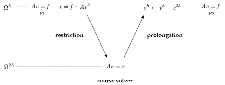
Coarse grid correction procedure involving \Omega^{h} and \Omega^{2h}.
Our First Multigrid Method: The V-Cycle
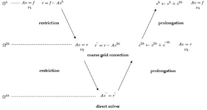
One question remains about the coarse grid correction: What if we don’t reach the desired error convergence on the coarse grid?
Let’s think about this for a moment. Solving the residual equation on the coarse grid is not at all different from solving a new equation. We can apply coarse grid correction to the residual equation on \Omega^{2h}, which means that we need \Omega^{4h} for the correction step. If a direct solution is possible on \Omega^{4h}, we don’t need to apply the coarse grid correction anymore and our solution method will look like a V, as shown in the figure below.
V-cycle multigrid solution method.
This solution method is called the V-cycle multigrid. It is apparent that multigrid methods are recursive in nature and a V-cycle can be extended to more than two levels. Coarse grid steps are quicker to compute than the fine ones and error will converge faster as we go down to them.
As it pays off to spend more effort on coarse grids, a method called W-cycle can be introduced where the computation stays on coarse steps longer. If the initial guess for the deepest V-cycle is instead obtained from shallower V-cycles, then we have what is called the full multigrid cycle (FMG). While the FMG is a more expensive approach, it also allows for faster convergence than just the V-cycle and the W-cycle.
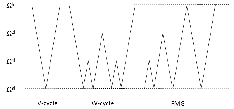
A plot comparing the V-cycle, W-cycle, and FMG.
Reviewing the Different Multigrid Methods
Here, we have presented the V-cycle, W-cycle, and FMG in their simplest forms. In order to solve complex multiphysics problems and reach optimal performances, multigrid methods are not used alone. They can also be used to improve the convergence of other iterative methods. This is what happens under the hood in COMSOL Multiphysics.
The techniques that multigrid methods piece together have been used for quite some time and are known for their limitations. The beauty of multigrid methods comes from their simplicity and the fact that they integrate all of these ideas in such a way that overcomes limitations, producing an algorithm that is more powerful than the sum of its elements.
Next Steps
- Check out the previous blog post in this series: On Solvers: Multigrid Methods
- Read A Multigrid Tutorial by William L. Briggs
Editor’s note: This blog post was updated on 4/18/16.

Comments (0)