
Guest blogger Anja Diez, a researcher in the Acoustics Group at SINTEF, shares a method for more efficiently modeling pulse-echo measurements in oil pipes.
Pulse-echo measurements are a standard application in the oil industry for detecting material properties behind pipes. The measurement setup is simple, but modeling is challenging due to the high frequencies of ultrasonic pulses and the complexities of 3D modeling for this type of application. A 2D axisymmetric simplification can be a valuable step that reduces computation time and allows for parametric studies. In this blog post, we discuss how we used this type of simplification to improve our pipe simulations.
Pulse-Echo Measurements in Pipes
In the oil industry, pulse-echo ultrasonic measurements are important for obtaining information about the material properties behind an oil pipe and about the bonding of the material to the pipe. Relevant considerations are, for example:
- What the quality of the cement behind the pipe is
- If the shale behind the pipe is bonded to the pipe
- If there is a fluid-filled gap between the pipe and the solid surrounding material
These considerations are important before and during production, but also during plug and abandonment operation when closing an oil field.
Pulse-echo measurements are used to derive the material properties outside of a pipe by measurements from inside the pipe.
From the circular transducer, a short Gaussian pulse is sent with normal incidence toward the pipe wall (Figure 1). Once the signal reaches the pipe wall, part of it is reflected back into the fluid toward the transducer while the other part is transmitted further through the pipe wall, to the outer material. The pulse is then reflected back and forth inside the pipe wall. Every time the pulse is reflected on the inner pipe wall part of the signal is transmitted toward the transducer.
These returning signals are recorded with the same transducer that is used to send the initial pulse. The decaying strength of the signal inside the pipe wall depends on the material parameters, specifically the impedances of the material inside the pipe, the pipe itself, and the material outside the pipe. The decay rate of this signal measured at the transducer can be used to estimate the material properties outside of the pipe if the properties of the pipe and the material inside the pipe are known.
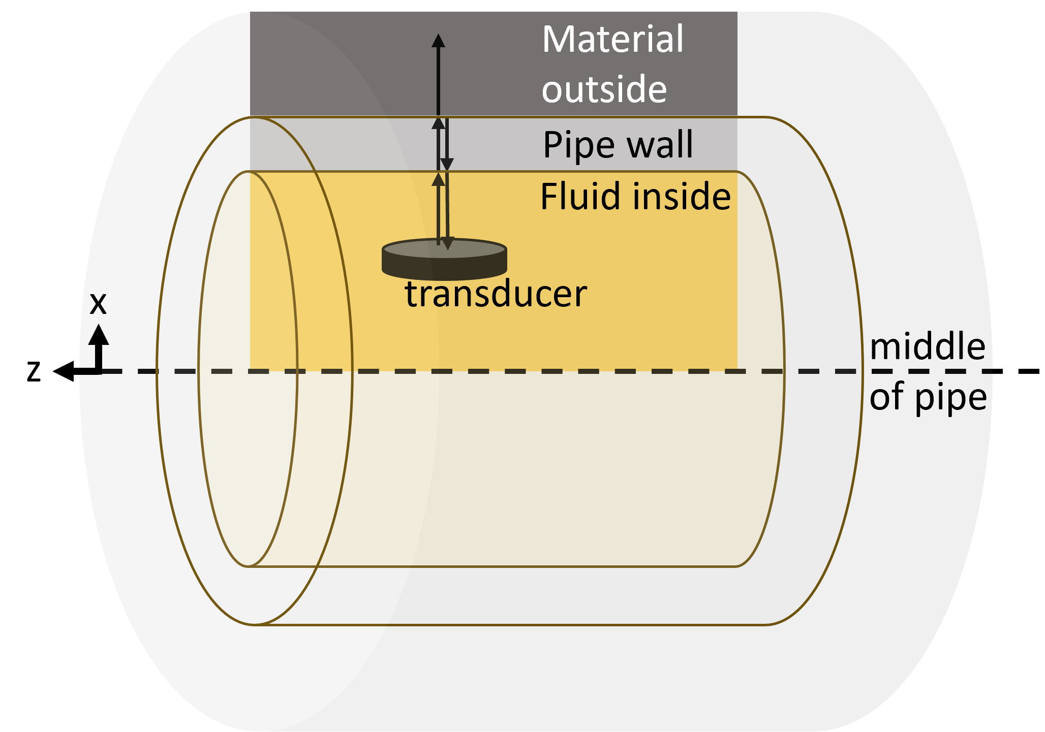
Figure 1. Concept of pulse-echo measurements in pipelines (left). An animation showing the transmitted and reflected signals (right).
Modeling this type of pulse-echo measurement in pipes is challenging due to the distance between the transducer and pipe, the high frequencies of the ultrasonic pulse, and the 3D geometric setup of a circular transducer within an elongated pipe. A 2D axisymmetric simplification is carried out with respect to the transducer symmetry axis, which proved to be a valuable step for the parametric study we were carrying out.
Through this model, we were able to reduce the computation time significantly, allowing us to build a database with about 1400 simulations including variations in pipe thickness and curvature, material parameters, and transducer–pipe distance, among other factors. These simulations allow for further research of the pulse-echo method, its sensitivities, and possible improvements to the interpretation of this type of data.
The COMSOL Model
To model this pulse-echo measurements setup correctly requires a 3D model. The transducer is circular, making it axisymmetric with the x-axis, while the pipe is axisymmetric with the z-axis (Figure 1). Hence, we can make use of two symmetry planes for this model, reducing the model domain to a quarter. Figure 2 shows the 3D model with the two implemented symmetry planes at four time steps. The ultrasonic pulse has propagated from the transducer surface (12 µs) to the pipe (36 µs), exciting acoustic waves in the pipe (52 µs), and the reflected pulse has traveled back to the transducer, where the signal is recorded (73 µs). Energy from the vibration within the pipe transmitted toward the transducer is visible behind the initial pulse in the snapshot at 73 µs. The modeling domain is surrounded by absorbing layers to ensure that no reflections of the waves occur at the domain boundaries. The xy-plane and the xz-plane are symmetric planes.
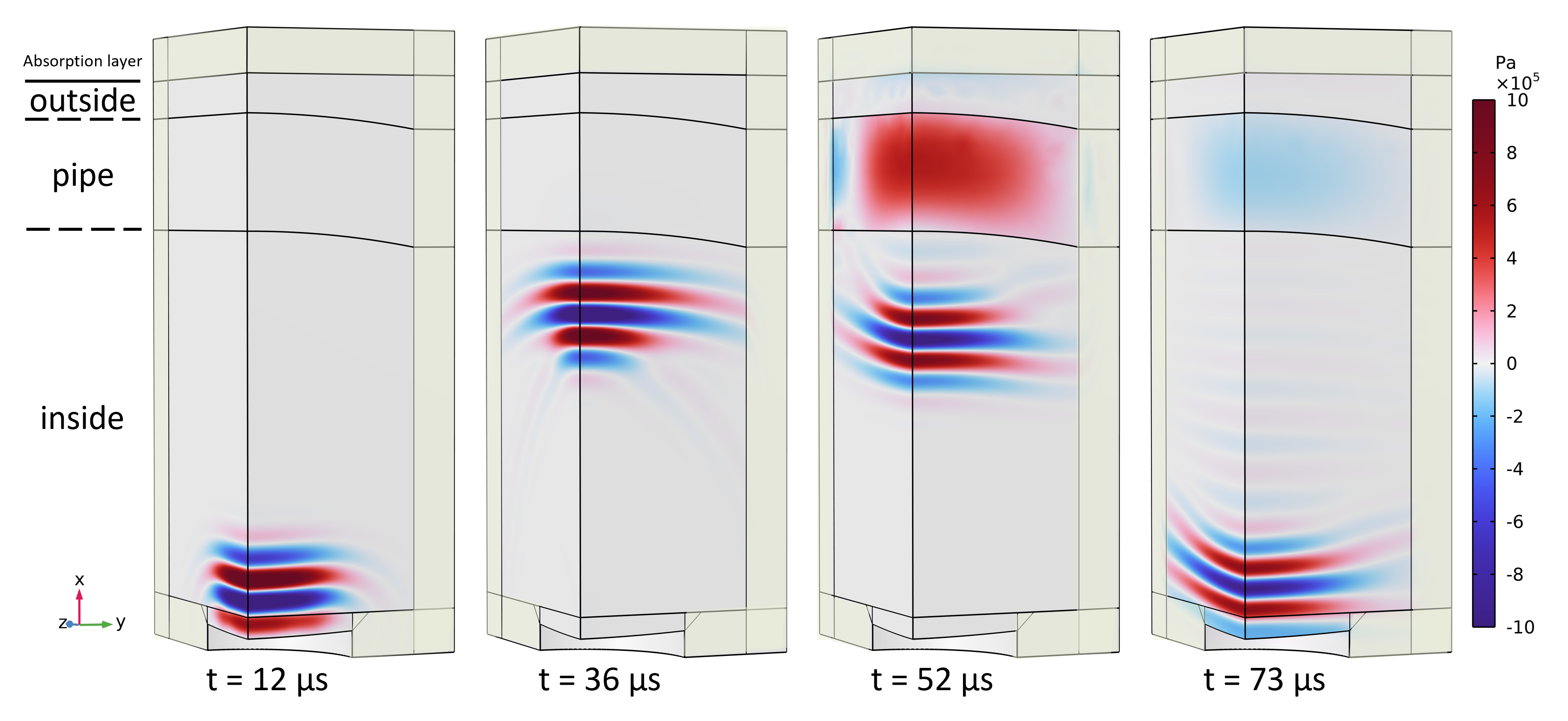 Figure 2. 3D modeling results at four time steps, making use of two symmetry axes.
Parameters of a standard pipe and transducer geometry, common in industry applications, were implemented for the model shown in Figure 2. These parameters can be found in the table below:
| Pipe Dimensions and Material Parameters |
|
|---|---|
| Material Inside Pipe |
|
| Transducer Parameters |
|
| Gaussian Pulse |
|
| Distance transducer |
|
The time-dependent study step is computed from 0 to 140 µs to allow the propagation of the ultrasonic pulse to the pipe and back as well as the recording of a significant part of the pipe’s reverberations.
Use of Time-Explicit Domain
The pipe in this model is normally filled with some kind of fluid. Here, we used oil-based mud with longitudinal wave velocities of 1301 m/s. The pipe itself is of steel, with a longitudinal wave speed of 5800 m/s. We calculated the element size for the mesh using:
with the element size h_{el}, the material’s wave speed v, and the maximum frequency f_{max}. Due to the large difference in the speed of sound in steel and oil-based mud, there are significant differences in the required mesh size for these domains. Figure 3 shows the mesh size for a 2D plane. The most efficient way to model this was by using the time-explicit mode. The acoustic domain of the fluid-filled pipe and the elastic wave domain of the pipe and surrounding material were then coupled by identifying the respective surfaces as identity pairs and using the Pair Acoustic–Structure Boundary multiphysics coupling.
The domain is surrounded by absorbing layers to prevent reflections from the domain boundaries. Here, two absorbing layers were defined, one for the acoustic domain and one for the elastic wave domain.
Geometry Reduction
To be able to carry out parametric studies with hundreds of variations, it is important to have a model with a relatively short computation time. Hence, using the 3D model with a computation time of more than 7 hours on our machine for each model is unrealistic. Therefore, we explored the possibility of reducing the geometry dimensions.
A standard way to reduce the computation time is by going from a 3D simulation to a 2D simulation. Taking a slice in the xy-plane and making use of the pipe’s mirror symmetry makes it possible to reduce the model significantly. In this 2D case, the pipe is modeled correctly, as the 2D model assumes infinite extend in the third direction. However, the source also becomes infinite in the third direction and is therefore not modeled correctly. This leads to significant deviations between the model results from 2D models compared to 3D models for this measurement geometry (Ref. 1).
Another possibility to reduce the geometry dimension is the use of a 2D axisymmetric model. As pointed out, the transducer is axisymmetric with respect to the x-axis, while the pipe is axisymmetric with respect to the z-axis (Figure 1). Here, we chose to carry out the axisymmetric model so that the symmetry axis aligns with that of the transducer (Figure 3). Thus, the geometry of the circular transducer is modeled correctly. Choosing again the xy-plane for the modeling of the 2D-axisymmetric part means we are modeling the curvature of the pipe. However, applying the symmetry about the x-axis means that the pipe curvature is assumed to be axisymmetric, hence modeled as a part of a spherical shell (Figure 4).
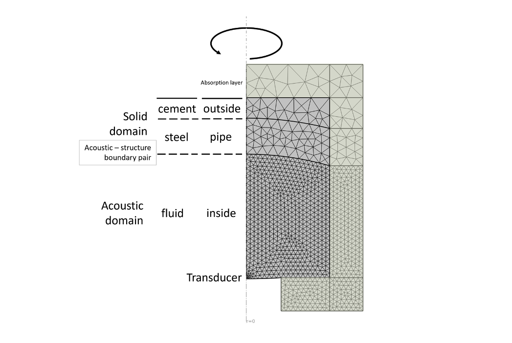 Figure 3. Building the model and grid for the 2D axisymmetric model. The time-explicit study step is used. The acoustic and solid domains are coupled by an identity pair.
Figure 4 shows the results of the wave propagation for the 2D axisymmetric model. The modeling is carried out for the domain shown in Figure 3, and the results in Figure 4 are plotted with the radial extension. The four presented time steps are the same as for the 3D model. The measured signal integrated over the transducer surface from the 2D axisymmetric and 3D model are plotted in Figure 5. (A detailed discussion of the comparison of 3D, 2D, and 2D axisymmetric models and the justification for using 2D axisymmetric models can be found in Ref. 1.)
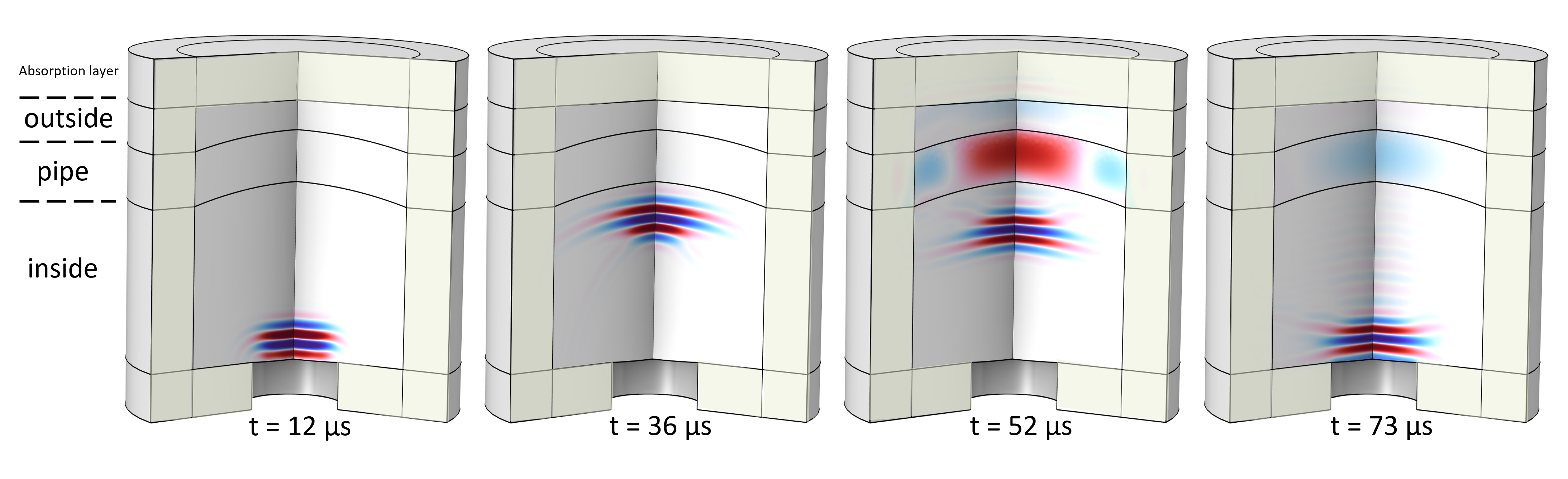 Figure 4. 2D axisymmetric modeling results in the revolved geometry for four time steps. The modeling domain is surrounded by absorbing layers.
Building a Database
The solution time for the 2D axisymmetric model was around 13 minutes, a significant improvement from the multiple hours of computation time for the 3D model. This speedup made it possible to build a database with hundreds of variations in the model (Ref. 2). Beside geometrical variations, we also introduced a fluid-filled annulus between the outside of the pipe and the surrounding solid material in the range of 10 to 1000 µm. We did this by making use of the advantages of the time-explicit implementation, using additional Pair Acoustic–Structure Boundary couplings for the transition between the fluid and solid domains. For each calculated model, the pressure at the transducer was exported and integrated over the transducer surface, giving the results of the measured signal from the pulse-echo modeling for further analysis and research (Figure 5).
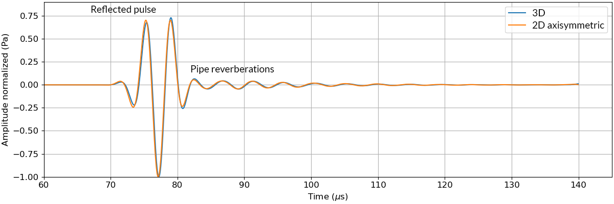 Figure 5. COMSOL model results of the pressure over the transducer surface.
To simplify the calculation of all these models, we used LiveLink™ for MATLAB®, which enables the integration of COMSOL Multiphysics® with MATLAB® By doing so, we were able to drive the variation of all the calculations we were interested in automatically and export the pressure over the transducer surface. The input information and the averaged pressure over the transducer surface were then written into a JSON file. These results make up the database, which can be used for further analysis.
Access the Data and Models
To further explore the model discussed in this blog post, download it via the following Application Exchange entry: Modeling pulse-echo ultrasonic data.
The data generated within this project, and the 2D axisymmetric and 3D COMSOL® models (v6.2), are available on Mendeley data (DOI:10.17632/3bs65nzpv2.1).
References
- A. Diez, T.F. Johansen, E.M. Viggen, “From 3D to 1D: Effective numerical modelling of pulse-echo measurements in pipes,” Proc. 46th Scandinavian Symposium on Physical Acoustics, pp. 1–23, 2023; ISBN 978-82-8123-023-1.
- A. Diez, E.M. Viggen, T.F. Johansen, “Ultrasonic pulse-echo dataset from numerical modelling for oil and gas well integrity investigations,” Sci Data 12, 544, 2025; https://doi.org/10.1038/s41597-025-04851-x
Acknowledgement
This work was a collaboration between A. Diez, T.F. Johansen (SINTEF), and E.M. Viggen (Norwegian University of Science and Technology) for the Centre for Innovative Ultrasound Solutions, funded by the Research Council of Norway under grant no. 237887.
About the Author
Anja Diez is a researcher in the Acoustics Group at SINTEF. She has a background in geophysics and worked the first years of her career using seismics and ground-penetrating radar to investigate the ice sheets in Antarctica and Svalbard, determining ice properties and conditions at the glacier bed. In recent years, she has worked on acoustic projects related to industrial applications and nondestructive testing, combining signal processing and data analysis with COMSOL® modeling for wave propagation in fluids and solids.


Comments (1)
Buraq Cfd
May 30, 2026Really appreciated this write-up — the geometry reduction approach is something I’ve been thinking about for a similar NDT application and this gave me a much clearer picture of how to justify the 2D axisymmetric simplification without losing physical accuracy.
The point about the transducer being axisymmetric with the x-axis while the pipe is axisymmetric with the z-axis is what makes this problem tricky, and I liked how you were transparent about the trade-off — modeling the pipe as a spherical shell section rather than a cylindrical one is an approximation, but the signal comparison in Figure 5 speaks for itself. The match between the 3D and 2D axisymmetric results is remarkably close given how much you’ve reduced the domain.
The speedup from 7+ hours to ~13 minutes per run is what really opens the door to building a database of 1400 simulations — that kind of parametric coverage would be completely impractical otherwise. I’m curious whether you observed any noticeable deviation between the two models at higher frequencies or for thinner pipe walls, where the curvature approximation might start to matter more?
Also great to see the LiveLink for MATLAB integration used for automating the parametric sweeps and JSON export — that workflow is underutilized in my experience and this is a good practical example of how much it can streamline large simulation campaigns.
Looking forward to exploring the dataset on Mendeley. Thanks for sharing the models openly — that’s genuinely useful for the community. BURAQ