

Advancements in AI promise large efficiency gains across various industries, including in areas of engineering, manufacturing, and scientific research. AI agents can take action, such as executing tasks in software tools, while keeping the engineer in the loop for important decisions, making agents well suited for iterative simulations and design studies. In this blog post, we will discuss how to set up a connection between an OpenAI™ Codex agent and the COMSOL Multiphysics® software and how to use the agentic capabilities to perform a nonlinear solver tuning for the purpose of speeding up a CFD simulation.
The Agentic Loop
Until recently, most AI-assisted workflows focused on conversational interfaces: Users asked the AI tools modeling questions and received generated code or guidance while remaining in control of each individual step. The Chatbot window in COMSOL Multiphysics® follows this paradigm, enabling engineers to ask modeling questions, generate and debug COMSOL API code, and streamline repetitive tasks, all within the software.
The next step in an AI-assisted workflow is moving from conversation to action. An AI agent can plan a sequence of tasks, execute them through software tools, inspect the results, and decide what to do next. In simple terms, an agent can be thought of as a wrapper or “harness” around a large language model (LLM). The harness applies the actions derived by the LLM. The LLM writes a piece of code and wraps it in a specific format to perform a tool call, which triggers the harness to, for example, open a command line and a command to run the piece of code.
Understanding Interactions Between Agents and COMSOL®
COMSOL Multiphysics® is a great fit for exploring the shift toward agentic workflows thanks to the COMSOL API, the software’s rich programming interface. Here, we will look at how agents can leverage the COMSOL API to assist engineers in their modeling workflows by acting as collaborators.
There are different ways to set up an agentic workflow in COMSOL Multiphysics®. For interactive workflows, it is recommended to use a client–server setup to inspect an agent’s progress and the state of the COMSOL model, which lives on a COMSOL Multiphysics® server (not to be mistaken with COMSOL Server™, an add-on product for deploying simulation apps). Both the COMSOL Multiphysics® user and the agent can connect to the COMSOL Multiphysics® server, see the model state, and make changes.
In a typical interaction between an agent and a live COMSOL model, the agent would:
- Generate the source code for a Java program using the COMSOL API for use with Java
- Compile and run the code using the Java commands bundled with the COMSOL Multiphysics® installation. Through the Java program, the agent would then:
- Connect to the COMSOL Multiphysics® server
- Query model properties, runs studies, and/or makes controlled changes
- Disconnect from the server
- Reason over the output, plan, and perform next steps
How to Connect COMSOL® and Codex
Now that we have covered the basics of how an agent interacts with a COMSOL® model, we’ll go over the steps for setting up an agentic workflow in the software.
Since we have an agent available, we won’t have to complete the setup manually. Instead, we can ask the agent for help based on the architecture description. To do this, we start with a COMSOL Multiphysics® server instance, connect the COMSOL® user interface (UI), and load a model. (Also see: Running COMSOL Multiphysics® in Client–Server Mode.) Then, we install and set up an agent. For this example, we will use Codex from OpenAI. Codex can create a skill that enables us to manipulate the model object located on the server. A skill bundles instructions and scripts in a package that you can reuse and share.
Here is the prompt we used to create a simple version of the skill:
Create a lightweight, local Codex skill named comsol-api. Install it as a repo-scoped skill. The skill lets Codex inspect and modify a COMSOL Multiphysics model located on a COMSOL Multiphysics server through the COMSOL API *for* use with Java.


The skill should work in a client-server configuration. The model is located on an already running COMSOL Multiphysics Server. The main part of the skill is a small wrapper script that compiles Java code using the COMSOL’s bundled Java compiler and API plugin classpath, and runs this program. The Java code should connect to the server, manipulate the model object and disconnect again. Before performing any changes, connect to the server and read the model tag.


Save the .java file of each agent interaction with the server in a workspace folder alongside a log of the output of the Java programs and the COMSOL progress log (showing computation time, memory requirement, degrees of freedom) for later reference.


Research here to learn more about the COMSOL API.


https://www.comsol.com/support/learning-center/article/overview-of-the-comsol-api-107912


Based on that, create an implementation plan and implement it. The skill should be intentionally light and only focus on running Java code against the already running server. No need for tests. Don’t install additional packages. Keep it package free.


Test the skill by adding a parameter and reading back the same parameter.
Luna — the most affordable current-gen OpenAI model, with a reasoning setting of medium — was able to implement a skill in under ten minutes.
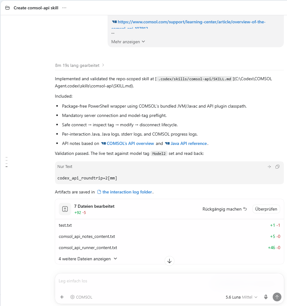 The Codex agent implementing and validating a skill.
To test the skill, the agent added a global parameter and then read the same parameter back from the live model on the COMSOL Multiphysics® server. During the test, the parameter appeared in the COMSOL Multiphysics® UI.
Possibilities and Challenges of Agents
Now that we have established a connection between COMSOL® and Codex, what can we do with it? Every click in the UI has a corresponding sequence of COMSOL API commands. Due to the comprehensive scope of the COMSOL API (which makes it possible to perform any part of the modeling workflow for any physics), Codex can perform any action.
The API can expose a broad variety of information for an agent to inspect, such as:
- Loaded model tags and component structure
- Parameters, expressions, descriptions, and units
- Feature types, labels, and tags
- Geometry and mesh sequences
- Physics interface and boundary condition settings
- Study and solver configuration
- Numerical results and evaluated expressions
- Warnings, errors, and solver logs
This information can be extracted, reasoned over, and manipulated, enabling agents to plan, run, and adjust experiments as necessary, as well as summarize the results in a report. This way, the agent can, for example, define parameters and settings, add physics interfaces, and create plots or numerical evaluations. Additionally, this agentic workflow enables you to perform sweeps that are usually not possible with the Parametric Sweep study. With the right setup, you can keep such a system running for an extended period of time.
Demonstration: Heat Sink Model
To demonstrate this capability, we will use the agent to experiment with nonlinear solver parameters in order to reduce the number of nonlinear iterations and speed up model computation, using the heat sink tutorial model as an example. The task is to analyze the available settings, select the three most promising ones, and run them with three values each. While the agent can traverse the model object and identify the corresponding node or search the COMSOL® documentation, we extracted the relevant code using the Copy as Code to Clipboard submenu to help the agent. This functionality is especially useful here, as the connection we implemented is quite bare bones. The prompt we used is as follows:
I am looking to speed up the computation, specifically reduce the number of nonlinear iterations necessary to achieve convergence. Analyze the parameters of the segregated solver, identify which might be good candidates to tune. Pick the most promising three and run three values each. Analyze the computation time, number of iterations in a report. Make only changes that are meaningful. I extracted the values that can be set in the segregated solver node.


model.sol("sol1").feature("s1").feature("se1").set("segterm", "tol");

model.sol("sol1").feature("s1").feature("se1").set("maxsegiter", 200);

model.sol("sol1").feature("s1").feature("se1").set("ntolfact", 1);

model.sol("sol1").feature("s1").feature("se1").set("segtermonres", "auto");

model.sol("sol1").feature("s1").feature("se1").set("segreserrfact", 1000);

model.sol("sol1").feature("s1").feature("se1").set("segstabacc", "segcflcmp");

model.sol("sol1").feature("s1").feature("se1").set("segcfltech", "interp");

model.sol("sol1").feature("s1").feature("se1").set("subinitcfl", 5);

model.sol("sol1").feature("s1").feature("se1").set("submincfl", 10000);

model.sol("sol1").feature("s1").feature("se1").set("subforcecfl", true);

model.sol("sol1").feature("s1").feature("se1").set("subkppid", 0.65);

model.sol("sol1").feature("s1").feature("se1").set("subkipid", 0.15);

model.sol("sol1").feature("s1").feature("se1").set("subkdpid", 0.15);

model.sol("sol1").feature("s1").feature("se1").set("subcfltol", 0.2);

model.sol("sol1").feature("s1").feature("se1").set("subadaptcfltol", true);

model.sol("sol1").feature("s1").feature("se1").set("segcflaa", "on");

model.sol("sol1").feature("s1").feature("se1").set("segcflaacfl", 9000);

model.sol("sol1").feature("s1").feature("se1").set("segcflaaset", "pid");

model.sol("sol1").feature("s1").feature("se1").set("segcflaadim", 10);

model.sol("sol1").feature("s1").feature("se1").set("segcflaamix", 1);

model.sol("sol1").feature("s1").feature("se1").set("segcflaadelay", 0);

model.sol("sol1").feature("s1").feature("se1").set("segcflaafact", 1);

model.sol("sol1").feature("s1").feature("se1").set("segcfljtech", "off");

model.sol("sol1").feature("s1").feature("se1").set("consistencycheck", "strictinitially");

model.sol("sol1").feature("s1").feature("se1").set("plot", "off");

model.sol("sol1").feature("s1").feature("se1").set("probesel", "none");
Your prompt can, of course, include additional resources, including Learning Center articles, blog posts, or Knowledge Base articles from the COMSOL® website.
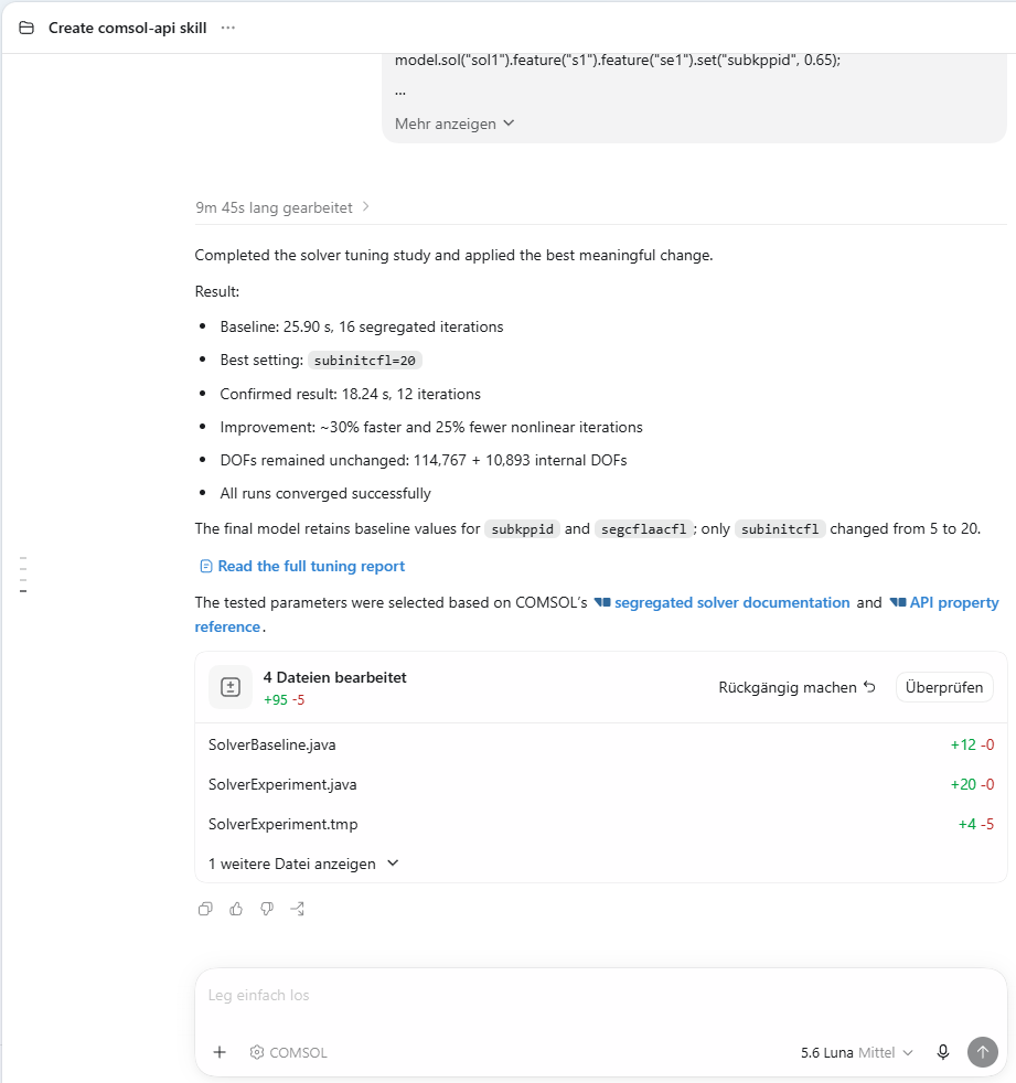 The results of the agent performing solver tuning studies.
Running nine experiments, the agent identified a relevant setting and reduced the number of nonlinear iterations by 25%, leading to a 30% faster computation time!
Another test we can run is to try out the difference between the three different comprehensibility options in the Laminar Flow interface. Although we cannot use the Parametric Sweep study in the UI to switch between the options in the dropdown menu directly, we can ask Codex to test each option, print the temperature in the chip, and list the number of nonlinear iterations. To instruct Codex to perform these tasks, here is the prompt we used:
There are three different compressibility options in the Laminar Flow interface. Run a test and compare all of them. I added an Evaluation Group that evaluated the temperature in the chip that you can run with the command:


model.result().evaluationGroup("eg2").run();


Create a report with the average temperature, computation time and number of iterations for the three different compressibility options.
There is no substantial change between the options, and the computation time is almost identical. So, we will stick with the default option. Please note that this was only an example on how to perform sweeps, and any settings in the interfaces should be taken based on physical considerations, not purely on computational speed.
Considerations When Using Agents
Although our experiments were successful, there are still challenges associated with agentic workflows. One of the challenges is spatial perception and spatial reasoning. For a human user, it is easy to select a boundary for a boundary condition by looking at the geometry. Under the hood, the number of the boundary is assigned to the selection of the respective boundary condition. Identifying this number purely by using the API can be difficult. Possible ways to circumvent this challenge is the rigorous use of named selections. Alternatively, you can activate the entity number in the view and instruct the agent to automatically export images from different view angles. This method is helpful as long as the geometry is not too complex.
It is also important to check the output to see if the changes are really meaningful. Considering the example of nonlinear solver tuning, the agent could simply change the termination technique to Iterations instead of Tolerance and set the maximum number of iterations to one. This method would reduce the number of iterations but would not give a numerically sound result. Monitoring key quantities, like the temperature of the chip, and ensuring that they do not change substantially is one possible way to filter out such bad candidates.
Since agents like Codex can do more than simply output text, there are risks associated with running them. They can make incorrect assumptions, delete files, expose sensitive data, or read malicious prompts on the websites they ingest. Because agents are inherently stochastic systems, they can make mistakes. To use these tools more safely, the agents should be operated in a sandbox, only have access to the files they really need, and require approval for high-risk actions.
Final Thoughts on Connecting Codex to COMSOL®
What we showed here is a minimal working example of a connection of Codex to COMSOL Multiphysics® for agentic workflows. This skill and wrapper script can be further extended to enable a more robust interface handling, which would be especially useful for identifying overly long simulation or mesh creation times for robust recovery.
These advancements can change how engineers interact with simulation software. The general scope of the COMSOL API makes COMSOL Multiphysics® well suited for updating simulation workflows to meet the era of AI.
OpenAI is a trademark of OpenAI, Inc. Oracle and Java are registered trademarks of Oracle and/or its affiliates.





Comments (0)