

Guest blogger Tobias Jonsson of Lightness by Design explores how coupled ASI modeling can be used to capture the influence of a surrounding fluid on the vibration response of a structure.
The vibration of structures is affected by the surrounding media. Air, one of these media, is light and compressible and thus can often be neglected when a structural engineer evaluates the vibration of a design. Simulations might be performed without a physical representation of the air — as if the structure were vibrating in a vacuum without any interference with a surrounding medium. Conversely, when a structure is submerged in water, with one thousand times the density of air and a higher speed of sound (stiffness), the water’s effect on the vibration characteristics is often noticeable.
Accounting for the Effects of the Surrounding Medium
Traditionally, this effect has been denoted “added mass”, derived from the following equation used to describe it.
In the equation, m is the mass of the structure, and m_{added} is the added mass. The value of the added mass has often been empirically derived by experiments where the eigenfrequencies of the structure have been measured in air and water, respectively. Eigenfrequencies, also known as natural or resonance frequencies, are the frequencies at which a structure naturally reinforces vibrations. The difference in eigenfrequencies is then used to calculate the added mass.
Unfortunately, this approach has led to the misunderstanding that the effect of the surrounding medium is an added mass that vibrates together with the structure, whereas actually, the surrounding media acts with a pressure on the surface of the moving object, and this pressure is highest when the surface speed is highest. Therefore, the pressure is not constant but changes in amplitude and direction depending on the direction of the moving surface.
The true influence of the surrounding fluid on the vibration response can be captured using COMSOL Multiphysics® and a coupled acoustic–structure interaction (ASI) modeling approach. Similar multiphysics simulations have been described in the blog post “What is the Best Way to Analyze Fuel Tank Vibration” and also in our blog posts on muffler design, such as “Evaluating the Effect of Shell Thickness on Muffler Performance“.
Simulating the Surrounding Media
The focus of this blog post is highlighting the effect of the surrounding media and clearly describing an alternative to “added mass”. The physical example used in this blog is a Kaplan turbine blade in a water domain. The effect on its frequency response from a varied gap to the pipe wall is studied. The figure below shows the full Kaplan turbine geometry and the considered gap. Note that pressure equalization at the leading and trailing edge of the blade is always possible, irrespective of the varied gap size.
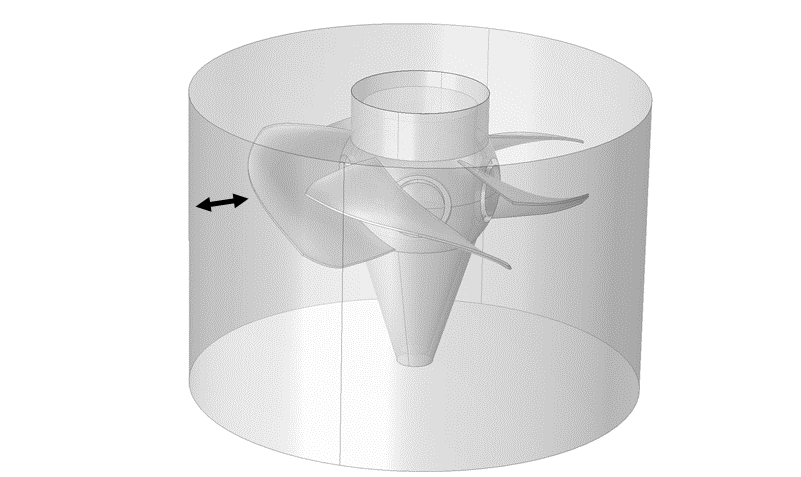 Kaplan turbine geometry with arrows showing the gap to the pipe wall.
Acoustic–Structure Interaction
The fundamental part of acoustic–structure interaction is the multiphysics coupling applied to the boundary between the fluid and the structural domain. The pressure degree of freedom (DOF) in the fluid is coupled to the three displacement degrees of freedom (DOFs) in the structure (in the x, y, and z directions), as described below.
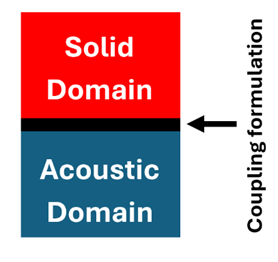
The conditions for an external boundary are
in which \bm{u}_{tt} is the structural acceleration (applied to the fluid), p_\textrm{t} is the total acoustic pressure, \rho_\textrm{c} is the density of the fluid (the subscript c indicates that this can be a complex-valued quantity used to model losses in the fluid ), \bm{q}_\textrm{d} is an optional acoustic dipole domain source term, \bm{n} is the surface normal, and \bm{f}_\textrm{a} is the (acoustic) load (force per unit area) on the structure.
The acoustic pressure is applied to the structural faces, and the acceleration of the surface is coupled to the acoustic domain. To enable the modeling of acoustic–structure interaction in COMSOL Multiphysics®, both the Pressure Acoustics, Frequency Domain and Solid Mechanics interfaces need to be added to the model. Furthermore, the multiphysics coupling described above needs to be enabled and added (under the Multiphysics node) to all boundaries between structural and fluid volumes. Here is how it looks in the Model Builder tree:
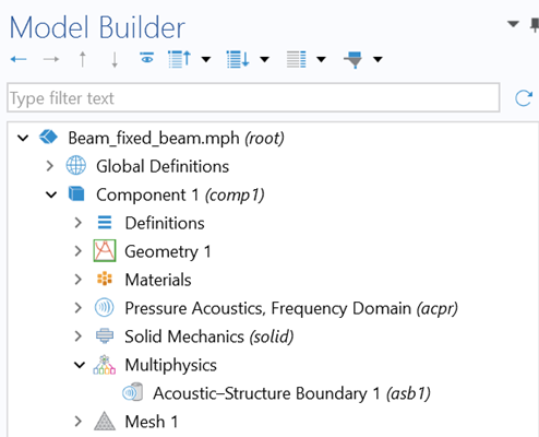 Building a vibroacoustic simulation.
As the problem is solved in the frequency domain, the model is assumed linear, and only small structural deformations can be modeled. Losses in the fluid can be accounted for in several ways using a fluid model or even more advanced boundary conditions such as the Thermoviscous Boundary Layer Impedance feature. Damping due to vorticity in a moving fluid, and even the effect of a moving fluid, requires solving a more advanced acrostic formulation such as the linearized Navier–Stokes equations, also available in COMSOL®.
Example Using a Kaplan Turbine Blade
In the following, the influence of the inner radius of a pipe has on the vibration response on the general Kaplan turbine, is investigated. With the functionality in COMSOL Multiphysics®, it is possible to apply periodic boundary conditions and only model one blade while capturing the effect of overlapping blades. The water volume is created by offsetting the circular sections at the top and bottom so that their connecting sides pass between the blades. On those sides, the periodic boundary condition is applied (shown as yellow in the figure).
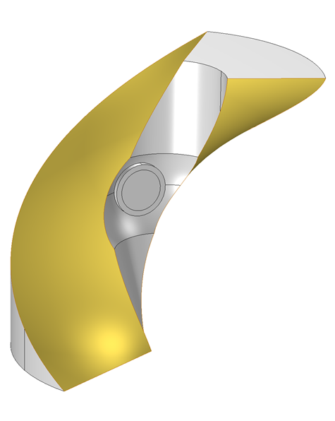
Water domain, with periodic boundary conditions in yellow.
The turbine blade was modeled as linear elastic with Young’s modulus 210 GPa, Poisson’s ratio 0.3, and density 7850 kg/m3. The water was assigned the properties of speed of sound at 1500 m/s and density at 1000 kg/m3.
For the model with a 10 mm gap to the pipe wall, 310,000 quadratic tetrahedral elements made up the mesh with refinements around the blade. The gap had at least 5 elements for all cases. The entire mesh was continuous, and no contact exists in the model.
All outer faces were set to the Sound Hard Boundary (Wall) boundary condition, which sets the normal component of the acceleration/velocity to zero. The condition is simply the natural Neumann condition for the total pressure, i.e., the normal derivative of the pressure is zero on the boundary
For the eigenfrequency analysis, the hub mount face of the blade was fully constrained
When determining the response to excitation in the frequency domain (the frequency response function, or FRF), an axial rotation of 1/\left(2\pi f\right)^2 rad/s2 was applied instead of the fully constrained boundary condition. That gives an acceleration of 1 rad/s2, regardless of the frequency.
Results of the Acoustic–Structure Interaction Analysis
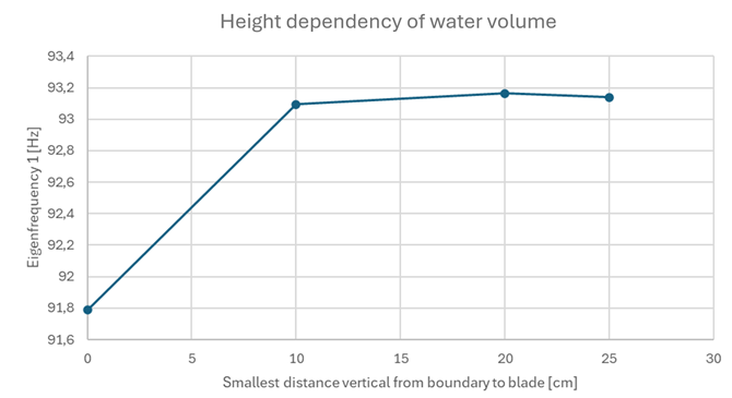
First, it was determined that the height of the water volume did not influence the results when the vertical distance between the blade and water boundary exceeded 10 cm above and under the blade. Therefore, this size of the water domain will be used throughout the study.
Second, the influence of the surrounding fluid (water or air) on vibration properties can be determined with the ASI approach. In the table below, the first six eigenfrequencies in water, with a gap large enough to not influence the turbine blade, are compared to the first six eigenfrequencies in free air. The table shows that water has a large influence on the eigenfrequencies, even when the gap has no effect.
| Blade in water [Hz] | Blade in air [Hz] |
|---|---|
| 104 | 193 |
| 148 | 262 |
| 279 | 442 |
| 753 | 1120 |
| 779 | 1202 |
| 980 | 1426 |
Finally, the influence of a varied gap size on eigenfrequencies can be determined. As the gap increases, eigenfrequencies do as well, up to a gap of about 150 mm. Here, eigenfrequencies converge to a constant value, regardless of a continued increase in gap size. The first six real eigenfrequencies for each gap size were derived and are presented below.
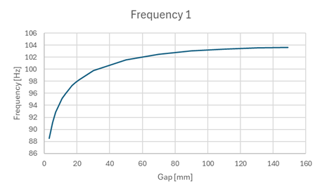
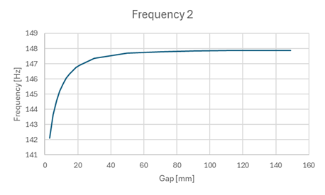
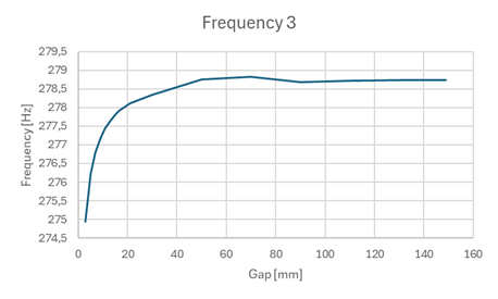
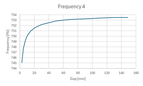
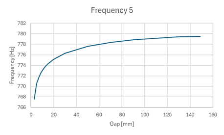
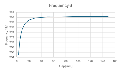
The first six real eigenfrequencies as functions of the gap.
The decreasing eigenfrequencies for smaller gaps can be explained by the increase in resistance for pressure equalization around the blade. It is not to be confused with damping from viscous effects, nor should it be simplified to an additional mass. Instead, we see how the water, modeled explicitly, affects the eigenfrequency of the system consisting of the turbine blade and water domain coupled together.
The corresponding mode shape for the fifth eigenfrequency for a gap of 149 mm is shown below, left. In COMSOL Multiphysics®, it is possible to plot the entire structure — not just the blade that is used in the calculation — giving a better overall picture of the state of the structure, as seen below, right.
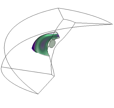
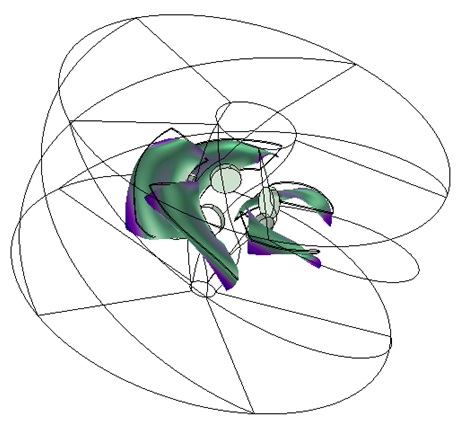
Mode shape 5 with a 149 mm gap, showing the blade used in the calculation (left) and the entire structure (right).
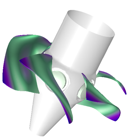 3D illustration of a Kaplan turbine propeller.
When the structure is instead excited by adding a frequency-independent rotation on the hub mount face of the blade, it results in the frequency-domain response presented in the figure below. Note that the frequency domain is swept in steps of 1 Hz and therefore the amplitude of the eigenfrequencies might vary depending on how close to the exact value is reached in this simulation. Regardless, peak response amplitude is not of the highest interest since it is most often desired to avoid these frequencies with some margin of safety in product development.
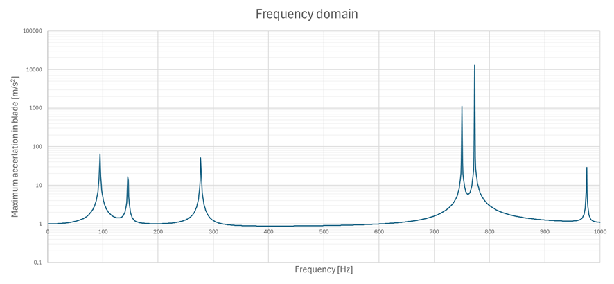 Acceleration response in the frequency domain.
Using functionality in the COMSOL Multiphysics® software, this example study has shown how modeling acoustic–structure interaction can be used to evaluate the frequency response for a structure submerged in fluid. This is an important step in the product development process for all products where the vibration response is a design criterion in the same way for underwater products as for products in air, where frequency analysis has been utilized for a long time.
In this example, it was made clear how the resistance of the flow of the fluid influences the frequency response of the structure in addition to the difference of submerging in water instead of in air. The eigenfrequency decreased by 57%, from 165 Hz to 71 Hz, by accounting for the surrounding water and minimizing the gap (to 3 mm).
Dynamic Loads on the Blade
A useful feature in COMSOL® is the Rotating Frame feature, which simplifies rotor dynamics by keeping your mesh stationary. By directly applying centrifugal, Coriolis, and Euler forces as body loads, it accurately simulates high-speed spin effects such as stress stiffening. This feature was not used in this example due to the low rotational speeds for this general application, but it is a powerful tool if the application requires it.
About the Guest Author
Tobias Jonsson is a structural mechanics specialist and consultant at Lightness by Design in Stockholm, Sweden. With an MSc from KTH Royal Institute of Technology, Tobias uses numerical simulation to help companies with simulation-driven product development. As part of a COMSOL Certified Consultancy, he is dedicated to integrating advanced simulation into the core of the product development process.
The consultants at Lightness by Design have contributed to the field of acoustic–structure interaction by coauthoring several research papers published in scientific journals. Furthermore, they have used their expertise in acoustic–structure interaction approaches to simulation and vibration design to help multiple clients in the product development process.





Comments (0)