Mount Erebus, one of Earth’s most remote volcanoes, sits covered in snow and ice. These chilly surroundings can be misleading, as Mount Erebus has another claim to fame: It’s the most active volcano in Antarctica. One option for mapping its magma flow is with a technique called magnetotellurics (MT), which measures the electrical resistivity of Earth’s crust. To study and improve MT, engineers can analyze its performance with electromagnetics simulation.
A Quick Introduction to Magnetotellurics
MT is a passive geophysical method that generates electrical resistivity profiles or reciprocal electrical conductivity profiles for specific areas of Earth’s subsurface and crust. This technique uses the natural electromagnetic source generated by the ionosphere.
When performing MT surveys, researchers often align the electromagnetic sensors by placing them in a line that runs perpendicular to an expected fault line or other anticipated strike of the formation. By simultaneously measuring the electromagnetic field as a function of time across different points in an area of interest, it’s possible to statistically evaluate the local electromagnetic impedance as a function of frequency. Using this impedance, researchers can predict the electrical resistivity as a function of depth.
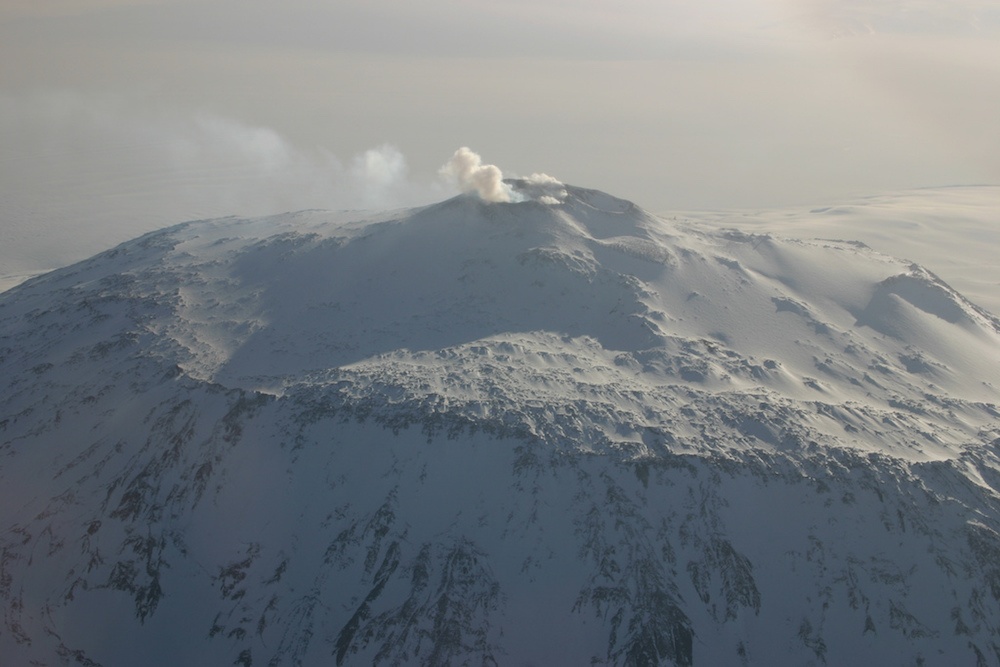
Mount Erebus, an active volcano studied with MT. Image by jeaneeem. Licensed under CC BY 2.0, via Flickr Creative Commons.
Since the rocks within Earth’s crust have different resistivities, the calculated profiles can help determine what types of rocks are located in a studied area — important information for scientists studying geological structures and processes. Besides rock composition, MT can also be used to investigate factors like porosity, permeability, and temperature.
Due to these abilities, MT has a quite a few different applications, including:
- Magma flow mapping for volcanoes
- Groundwater exploration
- Earthquake research
- Mining
- Geothermal research
- Petroleum exploration
To improve MT for these applications, the technique needs to be thoroughly analyzed and optimized. This is where simulation comes into play…
Using the AC/DC Module and Benchmark Data to Study MT
The model featured in this blog post represents a 70-by-70-km piece of Earth’s crust. It contains three “fault lines” along with three layers with different conductivities:
- 10-Ωm top layer
- 100-Ωm middle layer
- 0.1-Ωm bottom layer
There are two rectangular, high-conductivity inserts in the top layer of the model, where measurements are taken for real-world MT surveys. Using this model, you can estimate the conductivities of these inserts via the MT method.
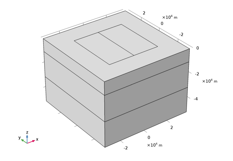
Geometry for the MT model.
To represent the magnetic field source, you can use a plane wave, which generates horizontal currents throughout the model geometry. Here, the MT analysis is based on the decomposition of the incoming plane waves into two waves that have perpendicular polarizations.
Note: While we don’t go into detail about setting up and solving the model in this blog post, you can find all of that information in the Magnetotellurics tutorial model. The accompanying documentation contains step-by-step instructions and you can even download the MPH file for this example as long as you have a COMSOL Access account and a valid software license.
The geometry and parameters for this model are taken from the study by Zhdanov et al. (ref. 1 in the model documentation) and the COMMEMI-3D-2 model, which is a benchmark for modeling MT.
Digging Into the MT Simulation Results
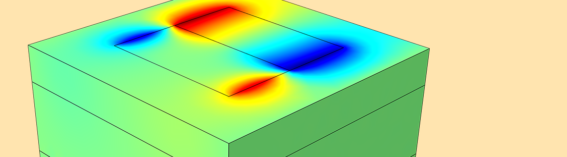
The first results show the components of the apparent resistivity, which can be extracted from the top layer and turned into surface plots for the analyzed frequencies. For uniform half-space or 1D models, the apparent resistivity at a specified position equals the resistivity below that point. Thus, at points where half-space approximations are valid, the apparent resistivity values should equal the material resistivity. This is because the skin depth is small at high frequencies. Below, you can see that locations with uniform resistivities that are far from fault lines have an apparent resistivity nearly equal to the resistivity of the material underneath them.


Top views of the logarithms of the apparent resistivity in the 3D domain.
Moving along, the next plot shows data from a line that crosses the fault lines in the model for two frequencies: 0.1 and 0.01 Hz. The results generated here are comparable with the reference literature. However, at lower frequencies, an increased discrepancy between apparent and material resistivity occurs.
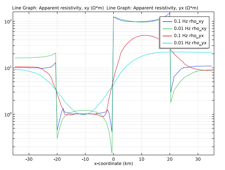
Apparent resistivity across strikes for frequencies of 0.1 Hz and 0.01 Hz.
Lastly is the tipper plot, where nonzero values indicate that there is a large variation in resistivity between the two sides of a fault line. By moving in the direction of the field vector at a certain phase value, engineers can use the tipper sign to determine if they are transitioning from a region with higher resistivity to a region with lower resistivity (where the tipper is positive) or vice versa (where the tipper is negative).
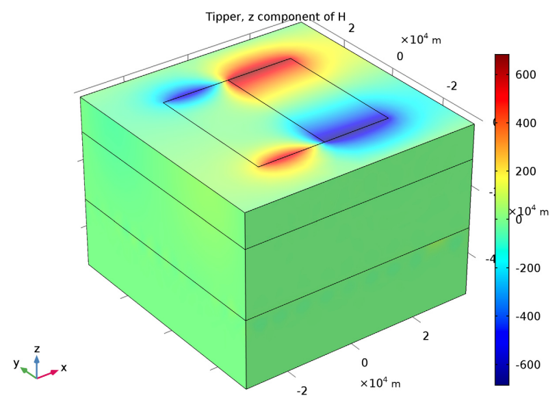
Tipper plot for a frequency of 0.01 Hz.
For simplicity’s sake, the model highlighted here only solves for two frequencies. However, MT data analysis is often gathered at frequencies ranging from 0.1 mHz to 10 Hz. It’s possible to add more frequencies to this study by adjusting the model size and mesh.
Next Steps
For more information about this example (or to try it yourself), click the button below.
Additional Reading
- Learn about other simulation studies that provide glimpses beneath the earth’s surface:


Comments (3)
Benozir Ahmed
June 20, 2018Dear Caty,
Thanks for the article. While working with Magnetic Field(MF) physics, if I scale down the geometry (Geometry>Length Unit> um) to micrometer then the solver fails to solve. I downloaded Magnetotellurics model and scaled all the dimensions from km to mm and the solver could solve. But If I scale it further down to um then the solver fails to solve. Do you know any solution to the problem? I will appreciate any suggestion.
Caty Fairclough
June 25, 2018Hi Benozir,
Thanks for your comment and interest in this topic!
For your question, I would suggest contacting our Support team.
Online Support Center: https://www.comsol.com/support
Email: support@comsol.com
Koustav Ghosal
July 31, 2021Dear Caty,
This article is very helpful. I would like to ask you about the weak form of the PDE used for the MT model. It will be great if you can share the equations with me. I will appreciate any suggestion from your side.