For transient acoustic problems, there are different sound pressure level metrics that have been defined in literature and in measurement standards. These metrics are important to know when comparing the results of a transient acoustic simulation to the measurements of a sound level meter or when trying to make results from a transient simulation easier to interpret on a logarithmic scale. Let’s take a look at what these different metrics are, when to use them, and how they can be computed.
Defining Sound Pressure Level
For steady-state harmonic noise, sound pressure level (\textrm{SPL}) is defined as:
where p_\textrm{rms} is the root mean square (RMS) pressure and p_\textrm{ref} is the reference pressure (e.g., 20 \mu \text{Pa} for air, also an RMS value). For a harmonic excitation with complex amplitude p:
where {}^* denotes the complex conjugate. Thus, \textrm{SPL} is well defined for steady-state noise and the expressions shown here can be used for computing \textrm{SPL} in the COMSOL Multiphysics® software using the Pressure Acoustics, Frequency Domain interface. Several variables are built-in for easy results analysis.
For transient noise, the RMS pressure over the entire time interval (T) could be computed as:
Since this expression averages over the entire interval, it’s not useful for comparing levels that change as a function of time during the interval. For this purpose, additional metrics can be analyzed. In this blog post, we will focus on:
- Computing Frequency Weighted pressure for a transient signal using the Window function capability in the Frequency to Time FFT study
- Computing Time Weighted Sound Level using a convolution in the time domain
- Computing Time Average Sound Level over a user-defined time period using a parametric sweep
Frequency Weighting
The human ear does not perceive the sound level of all frequencies equally. For example, the ear is much more sensitive to a 1000 \text{Hz} tone than to a 100 \text{Hz} tone. To mathematically account for this sensitivity when analyzing sound measurements, A-weighting was introduced as part of IEC 61672-1:2013. This is a function that adjusts the noise you are analyzing to compensate for the frequency.
Other weighting functions include:
- C-weighting: This is meant to capture the nonlinear response of the ear, such as changes in frequency-dependence for high sound levels.
- Z-weighting: This is a flat response, used to indicate zero weighting.
These three functions (A-, C-, and Z-weighting) over a normal frequency range are shown in the plot below:
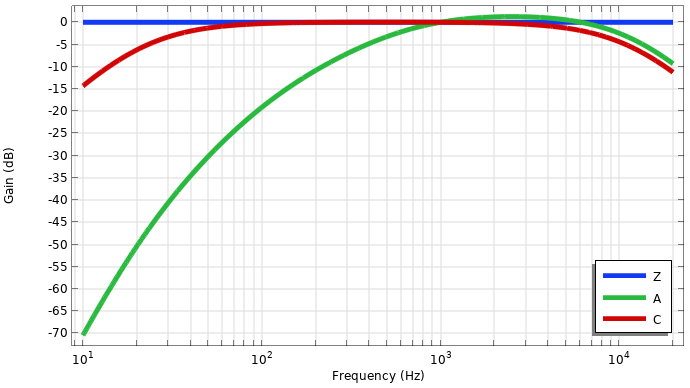
Plot of the A-,C-, and Z-frequency weighting functions.
The choice of weighting function is largely dependent on the application. For example, in the U.S., the Occupational Health and Safety Administration (OSHA) and Environmental Protection Agency use A-weighted metrics for occupational and environmental noise limits.
The A-weighted gain function is:
Here, f is the frequency and constants f_1=20.6, f_2=107.7, f_3=737.9, and f_4=12194. The function is defined to have 0 \text{dB} gain at 1000 \text{Hz}. Later, we will implement this function using parameters and an analytic function.
Note that the different types of weighting are built into the Octave Band plot. This plot is useful for postprocessing all frequency domain data. Tip: You can get a comprehensive introduction to this plot in our blog post “The Octave Band Plot for Acoustics Simulation”.
Time-Weighted Sound Level
Consider a time-dependent A-weighted pressure p_A(t). One could define an instantaneous sound pressure level in the following way:
However, there are some issues with this. First, when p_A(t) = 0, the resulting operation involves taking the logarithm of 0, so L_{p_A}(t) is undefined. A second, more practical issue dates back to when sound level meters were first being used. A needle indicator would move up and down to show the changing signal, as shown in the 3 side-by-side images below. Only, if we look at this with regard to the definition for instantaneous sound pressure level, there would be a problem: The needle would move back and forth so rapidly that it would be too difficult for the operator to see the reading at any given moment. (Ref. 1)


A sound level meter needle indicator.
To overcome this, the concept of time-weighted sound level was introduced. The definition is:
In this expression, \tau is the time constant and \zeta is an intermediate variable used for integration. The parameter \tau is defined to be 1 s for slow time-weighting and 0.125 s for fast time-weighting. Sound level meters manufactured to these specifications have slow and fast time-weight selections available to the user.
The time-weighted pressure is:
Let’s break down this expression. The function is a convolution of the squared pressure function and an exponential decay function. A convolution is a mathematical operation between two functions where they are multiplied and integrated. During this process, one of the functions is flipped and incrementally shifted along an intermediate axis, \zeta in this case. Let’s say we are using \tau = 0.125s for fast time-weighting with a pressure p_A(t) = \sin{\omega t} for an instant when t = \frac{6 \pi}{\omega}. We’ll visualize this by plotting both functions on the \zeta axis, normalized by the period T = \frac{2 \pi}{\omega}.


The individual functions in the convolution integral (left) and the integrand of the convolution integral, the resultant of multiplying them together at a discrete time (right).
When multiplying both functions together, what remains left for integration is a third function, which is nonzero only on a time interval that has been weighted by the current time stamp of the exponential function. It is clear that as time increases, more of the exponential function overlaps with the pressure signal, so one would expect the integral to increase up to a point for this case of the pure sinusoid.
Going back to the practical example, the time constant effectively slows down how fast the needle moves so the operator can actually read it as it is changing. Although its purpose before digital technology was for sound level meters, time-weighted sound level is still used today in current standards and sound level meters.
Equivalent Continuous Noise Level
Also defined in IEC 61672-1 is time-average sound level, also known as the equivalent continuous noise level. The definition is:
The averaging period T must be specified in reference to the measurement, but may represent any duration. The standard recommends the following integration times for sound level meters: T = 10 s, 1 min, 10 min, 30 min, 1 hr, 8 hr, or 24 hr. There is no convolution in this case; this is simply an RMS over a defined period.
The time-average pressure is:
The use of short averaging periods, on the order of seconds or shorter, is known as the short equivalent continuous noise level, or short Leq. This is useful for reducing data storage and transmission while still maintaining fairly high fidelity in the data for sounds recorded over long periods of time.
Example 1: Sinusoidal Pressure Signal
Frequency-Weighting
Here, we show a verification example that considers a simple sinusoidal waveform of constant amplitude and constant frequency. This can be implemented using an Analytic function with the expression P0*sin(2*pi*fdrive*t). We will use parameters to define a pressure amplitude of 1\text{Pa} and a drive frequency of 300\text{Hz}. The first step is to compute the A-weighted signal. We’ll add a second Analytic function for the A-weight that uses the parameters defined earlier.

The Settings window for the A weighting function.
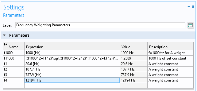
The settings window for Frequency Weighting Parameters.
We will add a 0D component and use a Global Equation in the Global ODEs and DAEs interface.
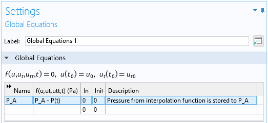
The Settings window for Global Equations.
Next, we can set up three study steps sequentially. First, the Time Dependent study is used to solve the equation defined in the image above, which effectively stores the signal as a dependent variable. Next, the Time to Frequency FFT study transforms the signal to the frequency domain. The last step (and the step involving frequency-weighting) is using the Frequency to Time FFT study step. Here, select the Use window function check box. For Window function, select From expression and insert the expression for the analytic function we defined earlier.

The Settings window for the Frequency to Time FFT study step.
The results from the study are shown below, zoomed into a few periods. The A-weighted pressure is in phase with the original signal, but with reduced amplitude. This reduction in amplitude can be verified by looking at the A-weighted frequency gain function curve, which shows ~-7 \text{dB} at 300 \text{Hz}. The gain can be computed by taking the logarithmic ratio of the amplitudes, i.e., 20 \log_{10} \frac{0.445}{1} = -7.03, which matches the curve.
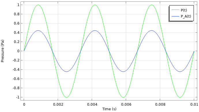
The result plot after using Frequency Weighting for the sinusoidal waveform.
Time-Weighting
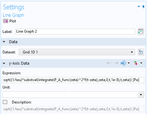
Now that the signal has been frequency-weighted, we will next compute the time-weighted pressure and time-weighted sound level. To begin, we will store the newly computed value of P_A(t) as an interpolation function whose data source is a derived value result table. This gives us a function for P_A(t), which is needed to compute the convolution.
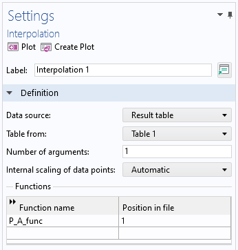
The Settings window for the Interpolation function.
To compute the convolution, a Grid 1D dataset is added. The expression used is shown below. In the expression, \zeta is the integration variable coordinate defined by the grid. t is a new variable introduced for the shifting of the exponential weighting function. The primary expression in substval() is integrate(P_A_func(zeta)^2*f(t-zeta),zeta,0,t,1e-8). This defines an integration over zeta from 0 to some varying quantity t, with an integration tolerance of 1e-8. substval() replaces t with a current value of \zeta, which allows the convolution to be computed.
The Settings window for computation of time-weighted pressure.
The results for the time-weighted pressure and sound level are shown below. Note that the signal must be resolved in time in order for the integration to be accurate. When the waveform is a pure sine wave, a few interesting things can happen. First, as time increases the fast-weighted pressure and fast-weighted sound pressure levels are approaching the RMS and overall sound pressure levels, respectively. For the pure sinusoid, the result can be checked against an analytical solution for the convolution integral that can be derived using integration by parts (multiple times). If the A-weighted pressure amplitude is P_{0A}, the analytical solution is
Furthermore, the time constant can also be interpreted as the time is takes to reach ~63% of the equivalent level. For example, 63% in dB is 10 \log_{10}{63/100} = -2dB. So, at t=\tau the time-weighted sound level should be about 2 dB below the equivalent level (about 84–82 dB for this case).


The result plots for time-weighted pressure (left) and sound level (right).
Time Averaging
The last step is to compute the time-average sound level. We’ll define parameters, including the averaging duration, number of averages, and moving upper and lower bounds for integration. A new Time Dependent study is added with a parametric sweep over the number of averages. The goal of this parametric study is to create moving upper and lower bounds that can be used for postprocessing. Note that no physics interface is actually solved here.


The Parameters (left) and Study (right) Settings windows for time-average computation.
The Line Segments plot can be used with the parametric solution dataset to plot the time average. In this plot, Solution parameters is changed to Manual, Parameter selection is changed to All, and Time selection is changed to Last. The line segment will span from the lower time to the upper time (x-coordinates) and the expressions (y-coordinates) is the calculation for time-average pressure, P_{AT}, and uses the timeint() operator.
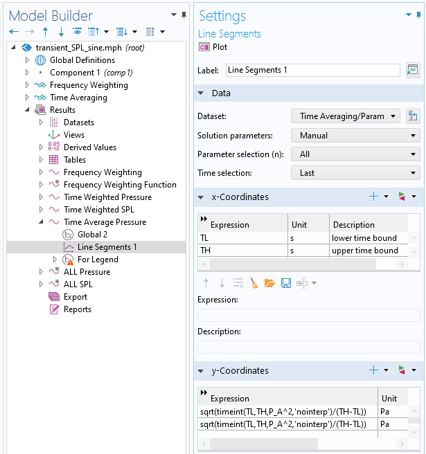
The Settings window for Line Segments for plotting the time-average pressure.
In this case, the averaging time is much greater than the period, so the time-average pressure is the RMS pressure. We can plot all of the results together for comparison.


The pressure versus time (left) and sound level versus time (right) results for the sine wave.
Example 2: Noise from Gearbox
In a previous blog post, we described how to model gearbox vibration and noise. Using the methodology described here, we can postprocess the noise and plot additional, useful metrics. To start, we will take the time-dependent pressure from a virtual microphone located at coordinates:
- x = 0.75 \text{m}
- y = 0 \text{m}
- z = 0 \text{m}
This data is loaded and stored in an interpolation function. The metrics are computed in the same way as the sine verification example.
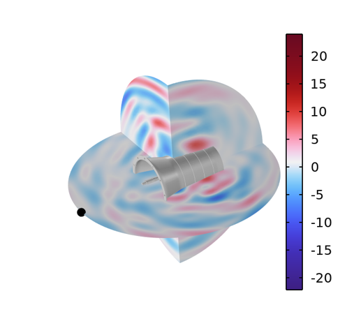
The acoustic pressure field around a dynamic gearbox. Time = 0.0020735 s.
For this example, we will use the fast-weighted constant, \tau = 0.125s. The averaging period will be T = 0.02s. The results show that the A-weighed pressure is amplified compared to the original signal. This is because most of the acoustic energy is in the 1000–3000 \text{Hz} frequency range.


The pressure versus time (left) and sound level versus time (right) results for the gearbox noise.
The results shown here are the A-weighted, time-weighted, and time-average pressures and sound pressure levels. These metrics are useful if, for example, you are trying to make results from a transient simulation easier to interpret on a logarithmic scale, are comparing the results to measurements from sound level meters, or are interested in how a transient signal would be perceived by the human ear.
Try it Yourself
Here, we have shown how to compute various transient acoustic metrics including frequency-weighting, time-weighting, and time-averaging. The definitions and main postprocessing steps outlined here can be used for any transient acoustic simulation. Try it yourself by clicking the button below, which will take you to the Application Gallery entry:
References
- E.H. Berger, The Noise Manual, AIHA, 2003.


Comments (1)
Daniel Smith
October 14, 2022Very nice and useful post, thanks for sharing.