

Have you ever wanted to compute the projected area of a CAD file? This can be useful in a variety of cases, such as for a quick estimation of the aerodynamic drag. There are several ways in which this can be done if you’re interested in the projected area along just a few directions, but what if you want to compute projected area over all possible directions? Here, we will look at an efficient way to compute and use such data.
A Couple of Simple Approaches
Let us consider a complicated CAD geometry. We start by asking: What is the projected area of this geometry along a particular direction? There are several ways of doing this. First, we can use the General Projection operator. This approach requires us to draw a box about the entire geometry and mesh very finely if we want to get good resolution. Due to the cost of meshing and integration over the entire domain, this approach can be quite expensive. The second approach, which is new in version 6.0, is to use the Projection of a 3D Model functionality, which lets us draw work planes in space and project the 3D CAD file onto that work plane. We can directly measure the areas of these projections. This CAD-based approach is much faster and does not require any meshing, but does require the CAD Import Module, Design Module, or LiveLink™ products. Both of these approaches are tedious if we want the projected area along many different arbitrary directions.
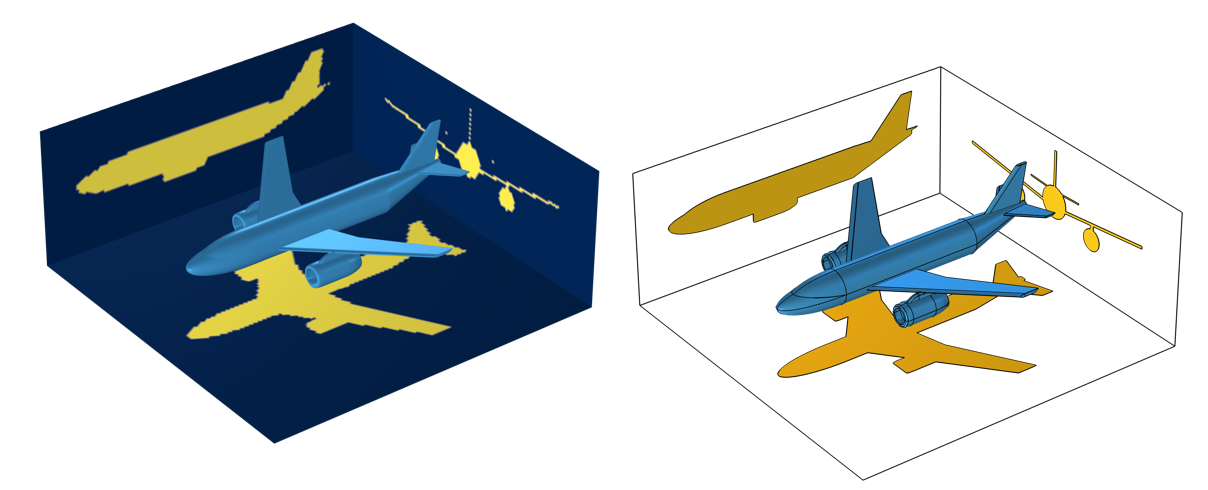
Two ways of determining projected area: via a General Projection operator, the results of which are mesh dependent (left), and with the Projection functionality, which creates projected surfaces onto a set of work planes (right).
A More General Approach
Rather than meshing the volume of the CAD file or adding CAD operations, we can exploit the definition of the projected area, which is:
where \beta is the angle between the line of sight and the normal to the surface, for those surfaces that are visible along that direction.
Taking a surface integral is very easy, but how can we evaluate the \cos \left( \beta \right) term? It turns out that we can get this term via the Surface-to-Surface Radiation interface, when we use an external radiation source of type Infinite Distance. Computing this requires solely a mesh on the surface of the part, not the volume. It does not even require solving for the surface-to-surface radiation as this incident external flux, with shadowing, is computed as a preprocessing step. So, we can simply integrate the external flux over all surfaces, divided by the nominal incident flux, and get the projected area along whatever direction that we have entered into the External Radiation Source feature. Since we use fourth-order Gaussian integration by default, a quite coarse mesh can be used.
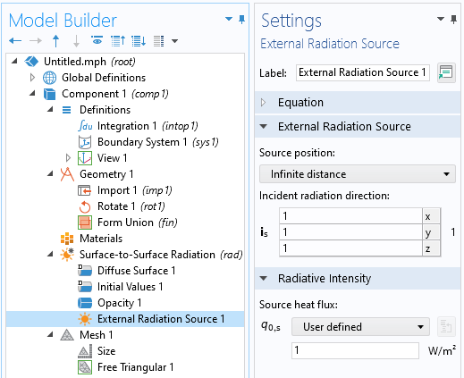
The External Radiation Source feature can be used to set up an illumination of a geometry to compute the projected area.
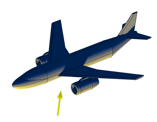
The incident flux, as precomputed via the External Radiation Source feature, can be integrated to get the projected area. Note the shadowing of the wing.
Extracting and Using Projected Area Data Over All Directions
It is often necessary to extract the projected area from all directions. Now, we could simply reevaluate the above integral for any incident direction of interest, but this would be quite expensive.
Instead, imagine a sphere surrounding the object, and choose a finite number of directions on that sphere from which to illuminate the target. Between those finite set of directions, we can then use linear interpolation over the entire sphere surface. But, before we choose these directions, it is worth remarking that the projected area is going to be symmetric about any plane through the center of the surrounding sphere, and that the CAD geometry that we are working with here is symmetric about the midplane, so it makes sense to exploit these two symmetries and only consider a quarter-sphere that lies in the positive xy-quadrant of space.
What we will go through next are the steps of:
- Creating a geometry, that exploits the symmetry of the CAD part, with a finite number of points defining the viewing directions
- Computing the projected cross-sectional area along those directions
- Interpolating the data onto all intermediate directions
- Extracting this data
To start, we create a very particular kind of geometry, as shown in the figure below. This geometry looks like a mesh of a quarter-sphere, and is created by first separately creating a mesh of part of a unit sphere, exporting that mesh, and then importing it into a second Component of the model. The import settings are such that each element of the surface mesh is a separate surface, and each node is a geometry point. This surface lies in the positive xy-quadrant of space.
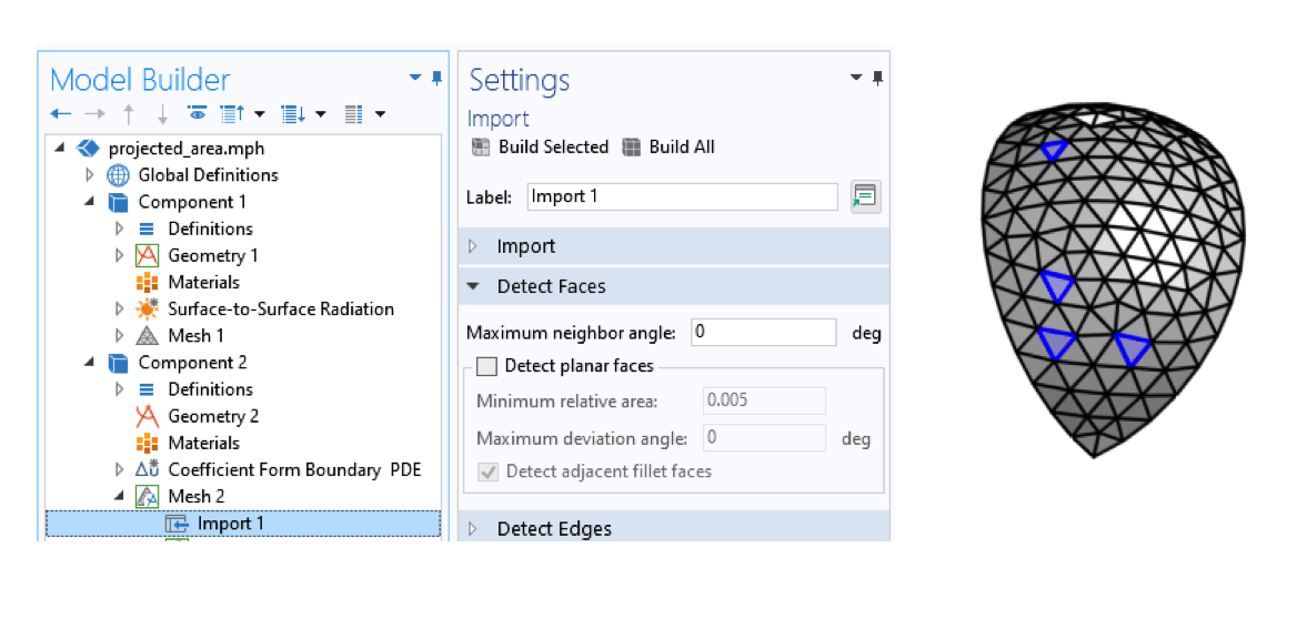
Importing a mesh with settings such that each element represents a different face.
Each one of these points is going to represent one of the sampled directions for which we will evaluate the projected area. Over each triangular patch between these points, we will linearly interpolate the area, using the linear finite element basis functions, so that we can approximate the projected area from any angle of incidence.
To this end, we add a Coefficient Form Boundary PDE over all of the surfaces of our quarter-sphere model, set the discretization to linear, and set the name of the dependent variable to AREA.
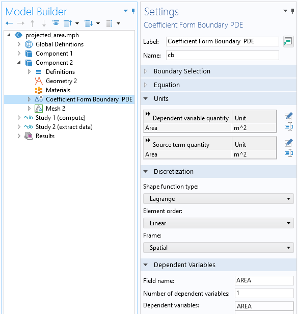
Settings for the Coefficient Form Boundary PDE interface that will implement interpolation.
Within this interface, we apply the Pointwise Constraint feature to all points in the geometry, which has the effect of totally constraining the problem, since all node points are at geometry points. The net effect of these settings is that all other physics settings have no effect and can be left at their defaults. The solution that we will get is just a linear interpolation between the constrained nodal values at the corners of each surface.
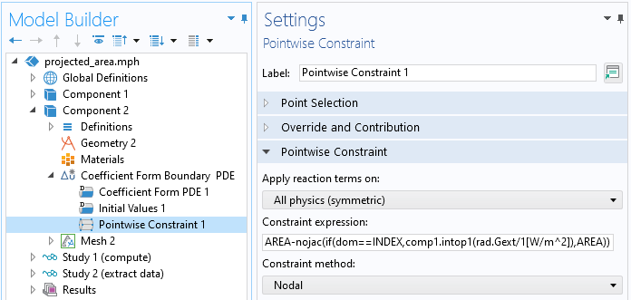
Applying the Pointwise Constraint to all points on a model.
We will therefore need to set, at each point, the projected area at that discrete viewing direction. To do so, we use the constraint expression:
AREA-nojac(if(dom==INDEX,comp1.intop1(rad.Gext/1[W/m^2]),AREA))
Let us unwrap this expression, which sets the value of AREA at each point. First, the entire expression must equal zero, so AREA is set equal to the expression within the nojac() operator. This operator means that the expression within it adds no Jacobian contribution, and for more details on this, see our blog post on accelerating model convergence with symbolic differentiation. Within this operator is the if(logical expression, true, false) statement. This statement starts with the logical expression dom==INDEX. Each geometry object (a domain, boundary, edge, or point) has a unique integer associated with it: its domain index, dom. Within the study we are about to run, we will run an auxiliary sweep over the global parameter INDEX for all points in this geometry.
During this sweep, when the logical expression evaluates to false, the AREA variable simply stays unchanged. When the logical expression is true, we get the projected area, the integral of the intercepted flux divided by the incident flux. The integration operator comp1.intop1() is defined within our first component over all exposed surfaces of the CAD file. However, when this integral is evaluated, how does the External Radiation Source feature in the first component know the direction associated with the point in the second component? We use a second integration coupling variable, over all of the points in the second component, and use that in the External Radiation Source direction field:
comp2.intop2(x[1/m]*(dom==INDEX))
The way to read this expression is: Evaluate over all points in the second component, the x-location (or y– or z-location), and multiply that by (dom==INDEX), which will be zero or one. That is, only for the currently indexed point will we evaluate the illumination vector oriented toward that point, as shown in the screenshot below.
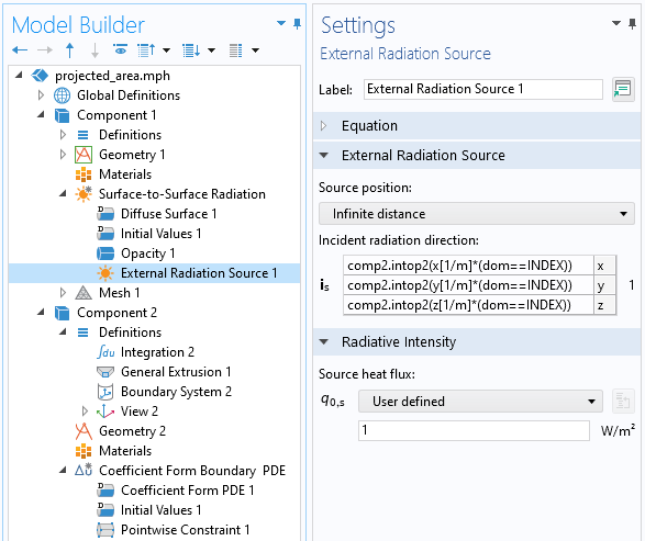
Within the first component, the incident radiation direction is set based upon the point locations defined by the geometry in the second component.
Next, we want to sweep over all values of our index variable, which we do via a Stationary Study Step that contains an Auxiliary Sweep. Within this study, we do not need to solve for the surface-to-surface radiation, since the incident flux is a preprocessing step.
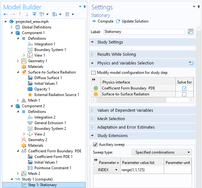
Sweeping over the index variable will get the projected area.
Since only the last value in the sweep contains all of the results, we can discard everything except for this last solution. This can be done via the Combine Solutions study step, as shown in the screenshot below.
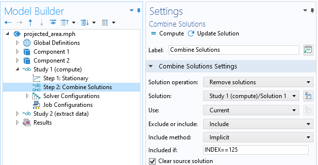
Using the Combine Solutions feature to keep only the last solution in the sweep.
Next, to give an example of how to use this data, we can use a second study with a Time Dependent step, where we will trace a point over the surface of the sphere in terms of a spherical coordinate system aligned with the airplane axis and upward direction defining the \phi and \theta angles.
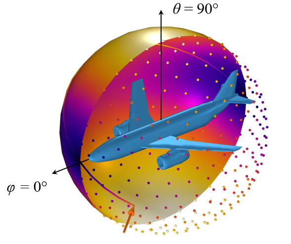
The CAD model and the projected area along discrete directions, represented by a set of points, as well as interpolated over a surface. The value of the field along a line traced over this surface can be evaluated via a General Extrusion operator in terms of a spherical coordinate system.
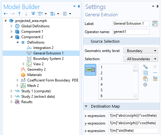
Extracting data from the interpolated data on the surface of the sphere via a General Extrusion operator.
To extract data from an arbitrary location on this sphere, in terms of a spherical coordinate system, we can use the General Extrusion operator as a dynamic probe by entering variables for the Destination Map expressions that account for the symmetry of the solution.
Closing Remarks
There are several ways you can compute the projected area of a CAD file. Of the three methods presented here, using the General Projection operator is the most computationally expensive, since it integrates over a domain and requires a fine mesh in the surrounding domain. Therefore, it should only be used if the other two approaches cannot be used. The second approach, using the Projection functionality, is a CAD-based operation. Although straightforward, accurate, and mesh independent, it requires manual setup for each projection direction. The last approach, using the Surface-to-Surface Radiation interface, is the most complex to set up but offers great flexibility in reusing data for further equation-based modeling. The file showing this approach is available for download here:


Comments (0)