
One of the more common questions we are asked is about the modeling of periodic, or pulsed, heat loads. That is, a heat load that turns on and off repeatedly at known times. Modeling such a situation accurately and efficiently in COMSOL Multiphysics is quite easy to do with the Events interface. The techniques we will introduce are applicable to many classes of time-dependent simulations in which you have changes in loads that occur at known times.
Editor’s note: This blog post was updated on October 4, 2022, to reflect updated modeling functionality.
A Brief Introduction to Time-Dependent Simulations
First, let’s take a (very) brief conceptual look at the implicit time-stepping algorithms used when you are solving a time-dependent problem in COMSOL Multiphysics. These algorithms choose a time step based upon a user-specified tolerance. While this allows the software to take very large time steps when there are gradual variations in the solution, the drawback is that using too loose of a tolerance can skip over certain transient events.
To understand this, consider the ordinary differential equation:
where the forcing function f(t) is a square unit pulse starting at t_s and ending at t_e. Given an initial condition, u_0=1, we can solve this problem for any length of time, either analytically or numerically.
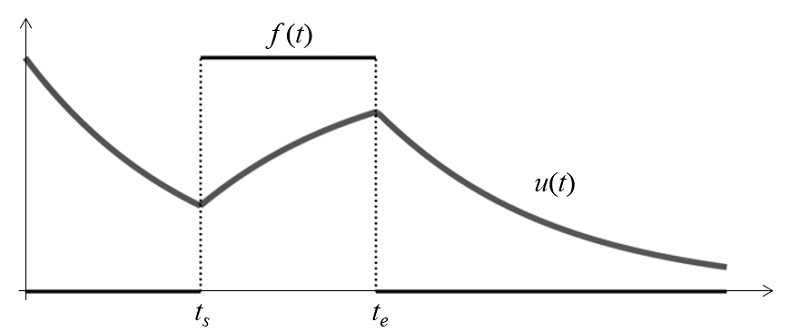
In the plot of the analytic solution (shown above), we can observe the exponential decay and rise as the forcing function is zero or one. Using the default time-dependent solver for this problem, let’s look at the numerical solution for two different relative tolerances:
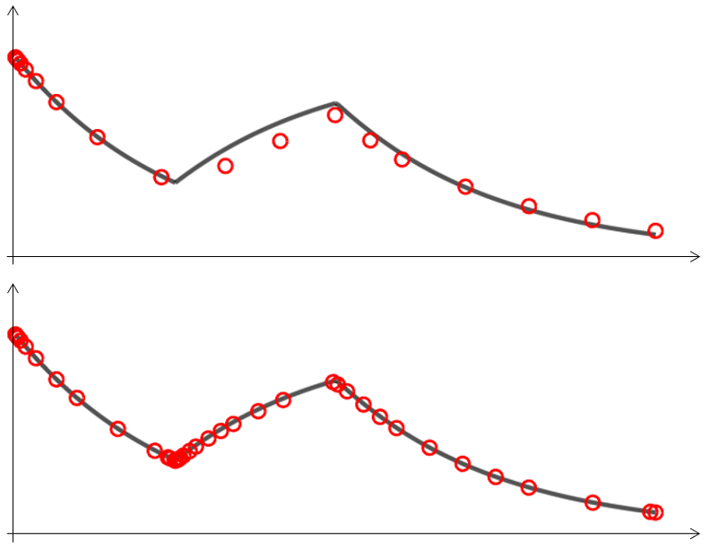
The numeric solution (red dots) is shown for a relative tolerance of 0.2 and 0.01 and is compared to the analytical result (grey line).
We can see from the plot above that a very loose relative tolerance of 0.2 does not accurately capture the switching of the load. At a tighter relative tolerance of 0.01 the solution is reasonably well resolved. We can also observe that the spacing of the points shows the varying time steps used by the solver. It is apparent that the solver takes larger time steps where the solution changes slowly and finer time steps when the heat load switches on and off.
However, if the tolerance is set too loosely, the solver may skip over the heat load change entirely when the width of the heat load gets very small. That is, if t_s and t_e move very close to each other, the magnitude of the total heat load is too small for the specified tolerance. We can of course mitigate this by using tighter tolerances, but a better option exists.
We can avoid having to tighten the tolerances by using Explicit Events, which are a way of letting the solver know that it should evaluate the solution at a specified point in time. From that point in time forward, the solver will continue as before until the next event is reached. Let’s look at the numeric solution to the above problem, with Explicit Events at t_s and t_e and solved with a relative tolerance of 0.2, a very loose tolerance:
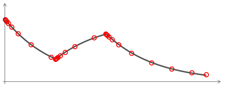
When using Explicit Events, the numerical solution — even with a very loose relative tolerance of 0.2 — compares quite well with the analytical result. Away from the events, large time steps are taken.
The plot above illustrates that the Explicit Events feature generates a time step whenever the load switches on or off. The loose relative tolerance allows the solver to take large time steps when the solution varies gradually. Small time steps are taken immediately after the events to give good resolution of the variation in the solution. Thus, we have both good resolution of the heat load switching on or off and we take large time steps to minimize the overall computational cost.
Now that we’ve introduced the concepts, we will take a look at implementing these Explicit Events.
An Example from Heat Transfer
We will begin with an existing example from the COMSOL Multiphysics Model Library and modify it slightly to include a periodic heat load and the Events interface. We will look at an example of the Laser Heating of a Silicon Wafer, where a laser is modeled as a distributed heat source moving back and forth across the surface of a spinning silicon wafer.
The laser heat source itself traverses back and forth over the wafer with a period of 10 seconds along the centerline. To minimize the temperature variation over the wafer during the heating process, we want to turn the laser off periodically, while the heat source is in the center of the wafer.
To model this, we will first introduce an Events interface and, within that, define a so-called Discrete State variable. The name of this variable is ONOFF, and it takes on an initial value of 1, as shown in the screenshot below.
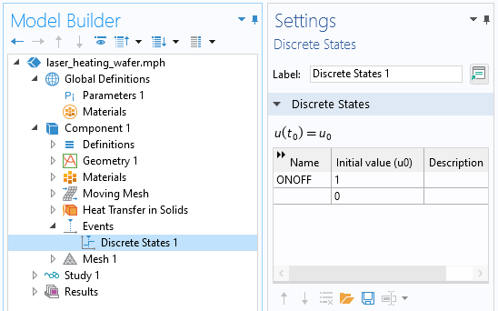
Screenshot of the Discrete States within the Events interface.
We can use this Discrete States variable to modify the applied heat flux representing the laser heat source, as illustrated below.
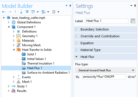
The settings for the applied heat flux boundary condition use the Discrete States variable.
So far, we are simply multiplying the applied heat load by a unit constant. Next, we can use two Explicit Events that can change the ONOFF variable. The first of these events will trigger initially at two seconds and set the ONOFF state variable to zero (turning off the heat load). It will repeat this every five seconds. The second will trigger at three seconds, turning the state variable back to one (turning on the heat load) — this will also repeat every five seconds.
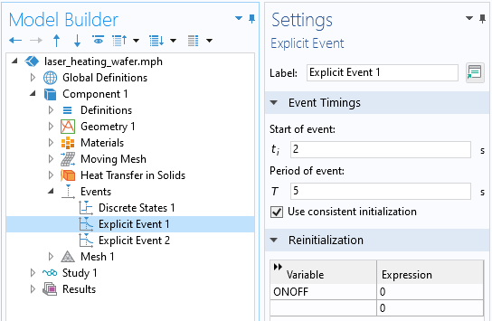
The Explicit Event settings. The first event has the effect of turning off the heat load. The second of these events starts at three seconds, and acts to turn the heat load back on.
No other changes are necessary, but we might want to ensure that we will get results immediately before and after each event is triggered. There are two settings that can ensure this, both shown in the screenshot below. First, you will need to open the Settings window for Time-Dependent Solver. There, in the Output section, you can enable the Store solution before and after events option. Alternatively, you can change the Times to store drop-down setting to Steps taken by solver.
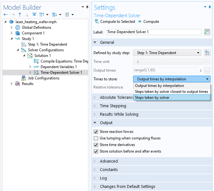
The Time-Dependent Solver settings for the storing of solutions before and after the events.
")
A comparison of unpulsed (left) and pulsed (right) heat loads.
You can compare the results of this simulation to the original model to see the differences in temperature across the wafer. With a periodic heat load, the temperature rise is more gradual and the temperature variations at any point in time are smaller.
Closing Remarks
We have looked at using the Events interface for modeling a periodic heat load over time and introduced why it provides a good combination of accuracy and low computational requirements. There is a great deal more that you can do with the Events interface — if you would like to learn more, please see our knowledge base article “Solving Models with Step Changes to Loads in Time”.


Comments (26)
Ivar Kjelberg
February 16, 2015Hi Walter
Thanks for an interesting BLOG again 🙂
One thing though: I do not read anything hereabove about the the relation between mesh density, that links to the material heat diffusivity “alpha” equal to k/rho/Cp and the time steps used.
If one does not also carefully consider these variables, there is a good chance that the errors you describe in the beginning are driven mostly by a poor mesh density.
I have noticed that you now propose the heat diffusivity “alpha” as a COMSOL internal variable, but I have not read anything that the mesher analyses this to adapt the mesh accordingly yet (automatically). Or have I missed a new feature ?
Sincerely
Ivar
Walter Frei
February 17, 2015 COMSOL EmployeeHello Ivar,
Yes, you are correct, one should always perform a mesh refinement study, as well as a study of the refinement of the time-dependent solver tolerance.
Do keep in mind that the advantage of the Events interface is that it will ensure proper temporal resolution of the periodic heat load, *regardless* of the mesh size or the time-dependent solver tolerance. Also, the first example presented here is a single degree of freedom problem, so there is no mesh dependency.
With respect to “alpha”: It appears that there are some misunderstanding here, and it is not particularly germane to this discussion about the usage of Events.
With respect to how you do the mesh refinement: You can perform either manual refinement or automatic adaptive mesh refinement. Adaptive mesh refinement in time-domain simulations has been available since several versions ago.
Best Regards,
Walter
Kiran Kabothu
July 20, 2015Dear Walter,
Thanks for your support.
I am working on ultra-short pulse laser matter interaction model in COMSOL (pulse duration <1ps).
In order to run simulation in time of 100fs, do i need the work station.
How i can chose the system configuration (processor, ram).
please suggest system requirement to solve my problem.
thanks
kiran
Walter Frei
July 20, 2015 COMSOL EmployeeHello Kiran,
Such questions should be directed to your COMSOL Support Team.
Best,
Sergey Fedotov
October 19, 2016Hello Walter,
Many thanks for your blog, it’s very usefull for me. I have a question related to using explicit events. I made a model which simulated material heating by one laser pulse and I did it by defining a initial temperature in focal spot. I wanted to simulate pulse train and added analytic function, two explicit events and multiply initial temperature in focal spot on analytic fucntion. Was it enough? Cause I expected to see graph T = f(t) like yours, but I didn’t.
Thanks for your reply!
Caty Fairclough
October 19, 2016Hi Sergey,
Thank you for your interest in this blog post! For questions related to your simulations, please contact our support team.
Online support center: https://www.comsol.com/support
Email: support@comsol.com
Best,
Caty
Melvin Lorenzo
December 10, 2016If I need to make pulses that are 100E-6 seconds in length, and they repeat once every second. How would I do this? I tried using this method but it doesn’t work for very small pulses.
Walter Frei
December 12, 2016 COMSOL EmployeeHello Melvin,
You may want to double-check your implementation, as this method does work for any pulse duration. You can confirm this by looking over the solver log.
Cory Cress
May 17, 2018You mentioned a flow-up blog post regarding alternative methods for dealing with instantaneous loads. Can you provide a link to that post, I can’t seem to find one that meets that description.
Walter Frei
May 17, 2018 COMSOL EmployeeHello Cory,
Yes, please see: https://www.comsol.com/support/knowledgebase/1245/
Best regards,
Cory Cress
May 22, 2018Thank you Walter!
The load I’m applying is a stepped load (like a staircase). Currently I’m using voltage = V_step*floor(t/period) to achieve this staircase. Because I’m using the floor function, I don’t believe the derivatives are continuous. How can I implement a staircase-like load that has continuous 2nd derivatives and is smoothed as you recommend? I’ve tried to use the built-in functions (i.e., step, analytic, piecewise) and combinations thereof without much success.
Along with my floor function, I’ve also defined events to occur at the same time as the voltage steps (i.e., my period). This was successful in making the voltage follow the staircase voltage profile as I defined (even when I reduce the tolerance to 0.1 – 2hrs to run). However, the current still increases non-physically beginning one or two time steps prior to the subsequent step in voltage (even with a tolerance of 0.001 66 hrs to run). I’m hoping that the smoothed load will help reduce this problem. If not, what should I do?
If I do implement the smoothed staircase, should I continue to use the explicit event? If so, when should I define the event? Should it be at the start of middle or end of the voltage step?
Finally, I’d like to run the data up to 50000 s, currently I’m running 1000 s with a step of 1 s. Increasing the length will increase the size of the results file which is already approaching 9 GB. Since I only care about the data just before and just after a step, how can I make the solver solve for those points only? During the voltage plateau, the system approaches a fairly steady state condition.
Thank you!
Scott Morrison
May 24, 2018Thank You Walter,
This is an excellent explanation, just what I was looking for.
I enjoy reading your blog.
Best Regards,
Scott
Giuseppe Turturiello
June 13, 2018Dear Mr. Frei,
thanks a lot for another great post. I like all your posts so far and they are extremely helpful. You mentioned that the alogrithms for solving time-dependent problems “choose a time step based upon a user-specified tolerance”. How does this looks like in a frequency-domain study? For example, suppose I have some high-frequency function within my model. How do I “feed” COMSOL with the correct information in order to avoid a kind of “aliasing”, i. e. COMSOL “sees” the function correctly?
Best regards,
Giuseppe
Walter Frei
June 13, 2018 COMSOL EmployeeHello Giuseppe,
You may find this article helpful in addressing your question:
https://www.comsol.com/support/knowledgebase/1245/
Best,
Giuseppe Turturiello
June 19, 2018Dear Mr. Frei,
thanks for your response.
Your posted link treats time-dependent studies. My question was about
frequency domain studies. Maybe I understood it wrong.
Kindly regards,
Giuseppe
Walter Frei
June 19, 2018 COMSOL EmployeeDear Giuseppe,
In the case of frequency domain models, you simply need to have a mesh fine enough to resolve the shortest wavelength in each material domain. See, for example, the modeling and meshing notes in this article: https://www.comsol.com/blogs/modeling-of-materials-in-wave-electromagnetics-problems/
maithem sabri
October 16, 2018Thank You Walter,
This is an excellent explanation.
Best Regards,
maithem
Muhammad Faraz
January 25, 2019Thanks a lot for good helping post. Can you kindly explain what is hf(x,y,t) in expression q0 of heat flux 1 settings window?
Regards
M Faraz
Walter Frei
January 25, 2019 COMSOL EmployeeHello,
You can find the example model here:
https://www.comsol.com/model/setting-up-periodic-heat-loads-for-simulation-46791
And you may also find this supplementary material helpful:
https://www.comsol.com/support/knowledgebase/1245/
Tran Hung
December 12, 2019Hello, I’m modeling pulsed laser heating. The problem is: the pulse duration is too small compared to the 1/repetition rate (4ns – 1/60 kHz), this made the calculation time too long. How can I simulate the laser heating in several pulse cycles?
Victor Martorelli
July 15, 2020Hello Walter,
Your blogs have been really helpful for what I require, thank you for that. Is it possible to use a supergaussian with similar parameters for the laser pulse? In extent a smoothed out square wave but that the peak is similar to the gaussian you described.
Thank you.
Walter Frei
July 16, 2020 COMSOL EmployeeHello Victor,
Based upon your question, you may find this model helpful:
https://www.comsol.com/model/laser-heating-of-a-silicon-wafer-13835
Poorvank Sharma
January 17, 2021Hi Walter,
Suppose we assume the flux is not periodic, then the events interface is not needed right?
Regards
Poorvank
Walter Frei
January 19, 2021 COMSOL EmployeeHello Poorvank, See also: https://www.comsol.com/support/knowledgebase/1245
Zain Haider
December 14, 2021Hi Walter,
Thank you very much for this helpful post.
I am working on a pulsed electromagnetic heating problem where I have evaluated the electromagnetic losses in frequecy domain and I am doing a transient thermal study. However, I would like to switch off and on the frequency domain electromagnetic losses in transient thermal simulations to get results for pulsed heating.
My specific question is how can I use the Events Interface to switch on or off the electromagnetic heating in Multiphysics coupling? Or is there some alternative way to achieve pulsed electromagnetic heating in COMSOL?
Currently, I am trying to manually couple the electromagnetic losses to bioheat heat module using Heat Source domain. In the Heat Source domain, I am multiplying the electromagnetic losses with an Analytic pulse to switch them on or off. In this case, I have disabled the Multiphysics coupling feature (electromagnetic heating) in COMSOL. However, I am not sure if it is the right way to do this.
I will be very grateful to you if you can please kindly help me and provide me some guidance regarding this problem.
Thank you,
Kind regards,
Zain
Walter Frei
December 14, 2021 COMSOL EmployeeHello Zain,
You can still use the Events. See also:
https://www.comsol.com/support/knowledgebase/1245
https://www.comsol.com/blogs/which-study-type-should-i-use-for-my-electrothermal-analysis/
https://www.comsol.com/support/learning-center/article/Introducing-Feedback-to-Models-of-Resistive-and-Capacitive-Devices-27111
https://www.comsol.com/support/learning-center/article/Functionality-for-Modeling-Inductive-Heating-in-Coils-9421/112