Problem Description
How should I model loads that change magnitude at a particular time?
I am solving a transient model which has loads that change instantaneously in time, but the solver appears to be missing some of these changes in the loads. How to I get the solver to correctly recognize when the load changes?
Solution
Background
Many time-dependent problems are modeled by partial differential equations with only first derivatives with respect to time. Common examples of such equations include the heat transfer equation and the chemical species transport equations, but any parabolic partial differential equation will behave similarly: the transient behavior of the solution is characterized by an exponentially decaying response to a change in the load. The default behavior of the software is to assume that the solution, and the applied loads, are smoothly varying in time. If, however, an applied load varies instantaneously in time, you should use the Events interface so that the software efficiently and accurately handles these changes.
If, on the other hand you model involves second time derivatives such as the transient electromagnetic wave and transient pressure acoustics formulations as well as transient structural problems, then the solution fields will be wave-like and such situations are addressed in Knowledge Base 1244: Solving Wave-Type Problems with Step Changes in the Loads
Resolution
Begin by adding the Events interface into the model. This interface is found within the list of Physics at Mathematics > ODE and DAE Interfaces > Events.
For modeling changing loads, the Events interface offers four different types of features: Discrete States, Indicator States, Explicit Events, and Implicit Events. When an event is triggered, by default it will consistently initialize all variables based upon the previous solution and new loads. You can, optionally, reinitialize some (or all) discrete states, global, or field variables to different values if you want them to change abruptly.
Periodically Pulsed Loads and Explicit Events
The Explicit Event feature should be used when you know the times at which a load changes, such as when modeling a pulsed load. It is typically used in conjunction with a Discrete States feature that is used to modify a boundary condition. You can also specify a Period of event to model regularly repeating changes in load. If a repeating pulsed load is applied, use two explicit events, one to trigger at the turn-on time, and the other to trigger at the turn-off time.
Consider, for example, a pulsed heat load that is on for one second, then turns off, with this cycle repeating every three seconds. This requires one explicit event to trigger when the heat load turns on, and another when it turns off. These events should repeat every three seconds, and they should modify the heat load. The modification of the heat load can be done via the discrete state feature, as shown in the screenshots below. A sample file implementing these features is also available for download via the link at the bottom.
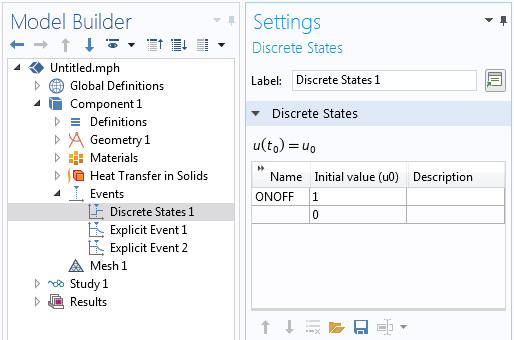
The discrete states interface defines a state variable that can be changed when an event is triggered.
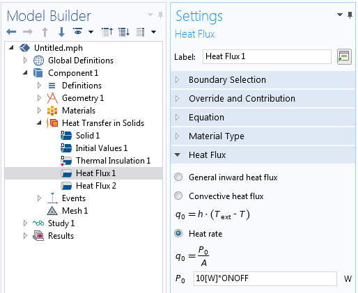
The discrete state can be used to modify a heat load.
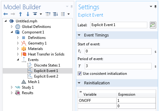
The explicit event reinitializes the discrete state, which turns on the load.
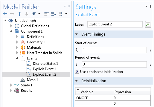
The explicit event reinitializes the discrete state to turn off the load.
Periodically Pulsed Loads without Events
If you have a load that is pulsing very rapidly relative to the simulation time-span, consider instead approximating this pulsed load as a cycle-averaged constant load.
For example, if you are modeling the heating due to a 10W load that is on for 100 milliseconds and off for 400 milliseconds over a total simulation time many times longer than the pulse cycle time, then it is quite likely that you do not need to explicitly model the temperature rise and fall due to each pulse. Instead, take the total time the load is on per cycle (100 milliseconds) and divide by the total cycle time (in this case 500 milliseconds) to get a 2W cycle-averaged heat load. This approach will solve much more quickly, especially for fast pulses, and is especially appropriate if you do not need to capture exactly the temperature rises due to each pulse.
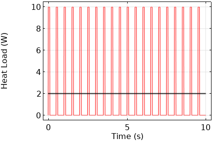
A constant, cycle-averaged, heat load (black line) over time can be a good approximation of the effect of a fast-pulsed load (red line.)
Conditionally Pulsed Loads and Implicit Events
The Implicit Event feature should be used when a change in load occurs implicitly due to a condition in the model that occurs at some unknown time, such as in the case of bang-bang, or thermostatic, control. It must be combined with an Indicator States feature, that defines an Indicator Variable. The indicator state variables are used to trigger implicit events when the indicator state variable changes sign and when the implicit event condition changes from false to true.
For example, consider a model initially at 20°C and being heated until the average temperature is above 95°C. At that point in time, the heater should turn off. The heater should turn back on if the average temperature drops below 90°C. A discrete state is used to control the heat load, as in the above example, but in this case the Initial Value setting is important. In this case, it must be initially one, indicating that the heater is on, and will be modified by the implicit events being triggered.
The discrete state is initially set to one.
To monitor the average temperature of domain within a model, use an average component coupling operator, as described in Knowledge Base 913: Computing Time and Space Integrals along with a variable that stores the average temperature, as shown in the screenshot below.
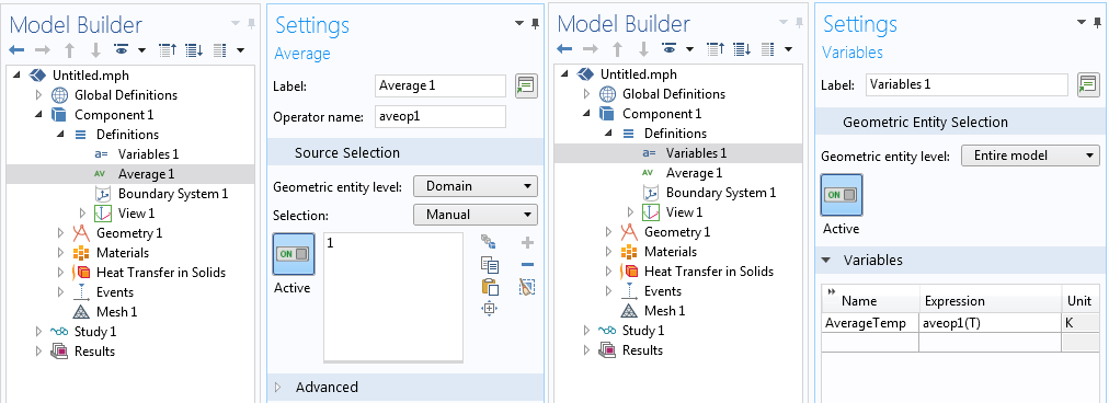
Defining a component coupling operator and a variable.
The monitored solution variable, in this case the average temperature variable, is used within the Indicator States features to define two indicator states that can cause an implicit event to trigger. The first indicator state defines TooHot = AverageTemp-95[degC] and the second defines TooCold = AverageTemp-90[degC]. Keep in mind that implicit events can only possibly be triggered when an indicator state changes sign.
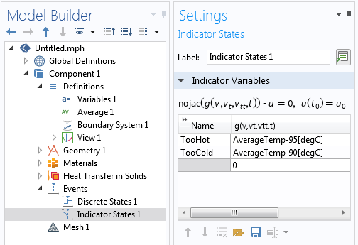
Defining the two indicator states.
The two indicator states are used within two different implicit events features, the first of which triggers on the condition TooHot>0 which goes from false to true when the average temperature goes above 95°C. When this event triggers, the ONOFF discrete state is set to zero, turning off the heat load. The second condition triggers on the condition TooCold<0 which goes from false to true when the average temperature drops below 90°C, and sets ONOFF to one, turning the load back on.
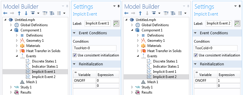
Two implicit events are used to implement thermostatic control.
The accuracy with which the solver will trigger Implicit Events is controlled by the Event tolerance, as shown in the screenshot below. If you are observing over- and under-shoots of the events, make this value smaller, 0.001 for example. A sample file implementing these features is also available for download via the link below.

Where to change the event tolerance.
Solver Options when using Events
By default the software will only save results at the times that you specify in the Time Dependent Study Step settings. You likely also want to store the solution immediately before, and after, any explicit or implicit events are triggered. This can be done by modifying the Time-Dependent Solver settings. Within the Output section, enable Store solution before and after events, as shown in the below screenshot.
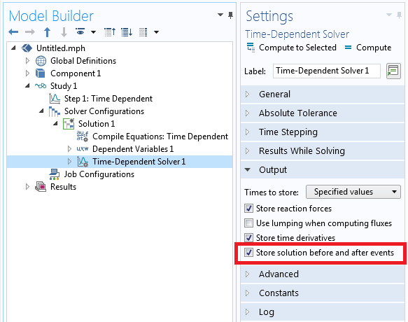
The solver settings that enable the storing of solutions before and after events.
See also:
Knowledge Base 1255: Reducing the amount of data stored in a model
Knowledge Base 1254: Controlling the Time-Dependent Solver Timesteps
Knowledge Base 1240: Manually Setting the Scaling of Variables
Knowledge Base 1127: Improving convergence in nonlinear time dependent models
Related Files
| pulsed_heat_load.mph | 748 KB |
| thermstat_controlled_load.mph | 804 KB |
COMSOL makes every reasonable effort to verify the information you view on this page. Resources and documents are provided for your information only, and COMSOL makes no explicit or implied claims to their validity. COMSOL does not assume any legal liability for the accuracy of the data disclosed. Any trademarks referenced in this document are the property of their respective owners. Consult your product manuals for complete trademark details.