

As of version 5.6 of the COMSOL Multiphysics® software, in the Semiconductor Module, we have introduced the capability of handling multicomponent wave functions to the Schrödinger Equation physics interface. Following the discussion in a previous blog post, we continue to explore this functionality using a model of a silicon quantum dot in a uniform magnetic field as an example.
Introduction to Quantum Dots
Quantum dots are an essential ingredient in nanotechnology with potential applications in solar cells, LEDs, displays, photodetectors, and quantum computing. One of the papers on the last application area is published by Jock et al. (Ref. 1) on the topic of spin-orbit qubits. In the Supplementary Note 1 of the paper, the authors provided the formulation describing a silicon quantum dot in a uniform magnetic field and showed the numerical solution in Supplementary Figure 1, which will be reproduced by this model.
The Formulation
Equation 1 in the Supplementary Note 1 of Ref. 1 gives the single-electron Hamiltonian for a silicon quantum dot in a uniform magnetic field \mathbf{B}, without including spin-orbit coupling:
(1)
+\frac{P_y^2}{2 m_\perp}
+\frac{P_z^2}{2 m_\parallel}
+V(\mathbf{r})
+\mu_B \mathbf{B} \cdot \sigma
where m_\perp and m_\parallel are the effective masses in the lateral and vertical directions, respectively; V is the confinement potential energy of the quantum dot; \mu_B is the Bohr magneton; \mathbf{\sigma} is the vector of Pauli matrices; the gyromagnetic ratio tensor is assumed to be a scalar of value 2 following the paper; and the kinetic momentum \mathbf{P} is given by
(2)
where e is the elementary charge, \mathbf{A} is the vector potential given by \mathbf{A}(\mathbf{r})=\frac{1}{2}\mathbf{B}\times\mathbf{r}, and there is no minus sign in front of the imaginary unit i because all physics interfaces in COMSOL Multiphysics take the engineering sign convention of exp(-i k x + i \omega t) instead of the physics sign convention of exp(i k x – i \omega t).
The confinement potential energy term V(\mathbf{r}) is given by Eq. 9 in the paper:
(3)
+\frac{1}{2} m_\perp \omega_y^2 y^2
+q F_z z
+U_0 \Theta(z)
where the first two terms represent an anisotropic harmonic trapping potential in the lateral directions with trap angular frequencies \omega_x and \omega_y in the x– and y directions, respectively; the third term describes an electric field F_z in the z direction; q is the particle charge (q=-e for electrons); and the last term is a potential barrier of height U_0 at the silicon-oxide interface at z = 0.
Parameters and Variables
The modeling parameters are shown in the table below:
| Name | Expression | Value | Description |
|---|---|---|---|
| mxy | 0.19*me_const | 1.7308E-31 kg | Lateral effective mass |
| mz | 0.98*me_const | 8.9272E-31 kg | Vertical effective mass |
| wx | 1[meV]/hbar_const | 1.5193E12 rad/s | Trap frequency in the x direction |
| wy | 3*wx | 4.5578E12 rad/s | Trap frequency in the y direction |
| Fz | 10[MV/m] | 1E7 V/m | Electric field |
| U0 | 3[eV] | 4.8065E-19 J | Oxide energy barrier |
| uB | e_const*hbar_const/2/me_const | 9.274E-24 m2·A | Bohr magneton |
| B | 1[T] | 1 T | Magnetic flux density |
All parameters are given in the paper, except the magnetic field, for which a guess value of 1[T] is used.
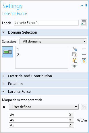
The vector potential \mathbf{A}(\mathbf{r})=\frac{1}{2}\mathbf{B}\times\mathbf{r} is specified using variables, assuming the uniform magnetic field points in the y direction:
| Name | Expression | Unit | Description |
|---|---|---|---|
| Ax | z*B/2 | Wb/m | Vector potential |
| Ay | 0[Wb/m] | Wb/m | Vector potential |
| Az | -x*B/2 | Wb/m | Vector potential |
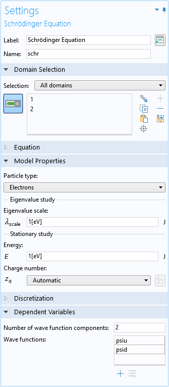
Physics Settings
The Schrödinger Equation physics interface is set up with two wave function components, psiu and psid, for the spin-up and spin-down components, respectively:
The default Effective Mass domain condition is used to specify the lateral and vertical effective masses:
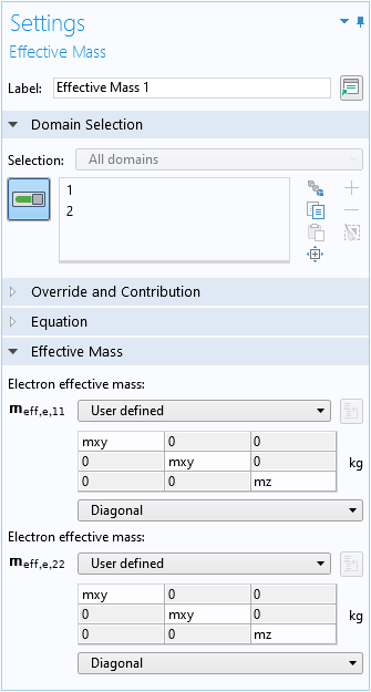
Even though, in this model, the two wave function components share the same effective masses, the user interface allows different values for different wave function components for general cases.
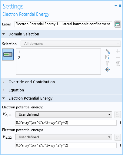
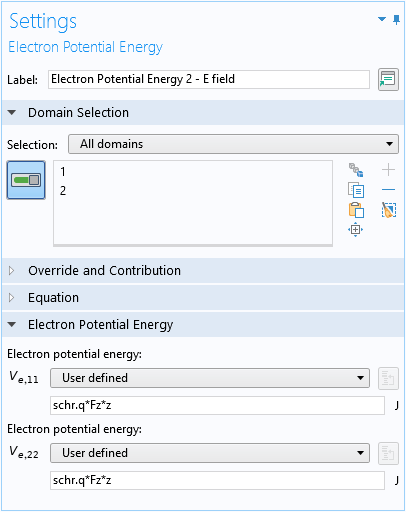
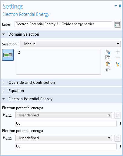
Three Electron Potential Energy domain conditions are used to set up the confinement potential energy term V(\mathbf{r}) (Eq. 3) for the lateral harmonic trapping:
For the electric field:
For the oxide barrier:
The contribution to the kinetic momentum from the vector potential (the second term in Eq. 2) is implemented using the Lorentz Force domain condition:
Finally, the magnetic coupling of the spin-up and spin-down components (the last term in Eq. 1) is implemented with the Zeroth Order Hamiltonian domain condition:
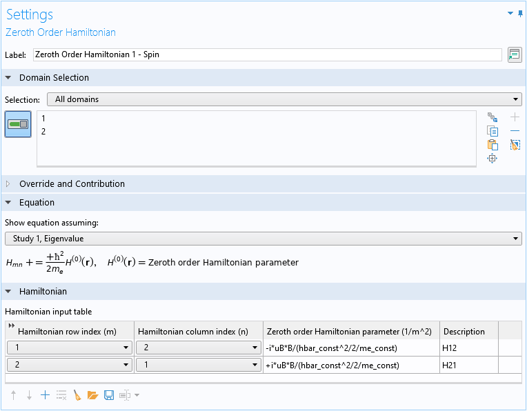
Note that the factor of \hbar^2/2m_e assumed by the domain condition should be compensated in the inputs, so that the net result is the last term in Eq. 1:
(4)
= \mu_B B \, \mathbf{n}_y \cdot \mathbf{\sigma}
= \mu_B B \sigma_y
= \left( \begin{array}{cc}
0 & -i\, \mu_B B \\
+i\, \mu_B B & 0 \end{array} \right)
In the screenshot above for the Settings window of the Zeroth Order Hamiltonian domain condition, the first row of the Hamiltonian input table implements the (1,2) element of the matrix in Eq. 4, and the second row implements the (2,1) element.
A simple swept mesh is created and an eigenvalue study is used to find the first few eigenstates.
Understanding the Results
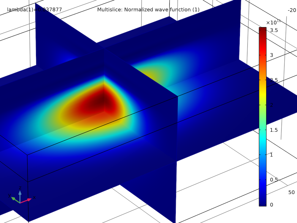
By plotting the real and imaginary parts of the spin-up wave function component of the first two eigenstates, we find that they have similar magnitudes and shapes, except for some sign flips:
| Spin-Up Wave Function Component | |
|---|---|
|

|
| Ground state, real part | Ground state, imaginary part |
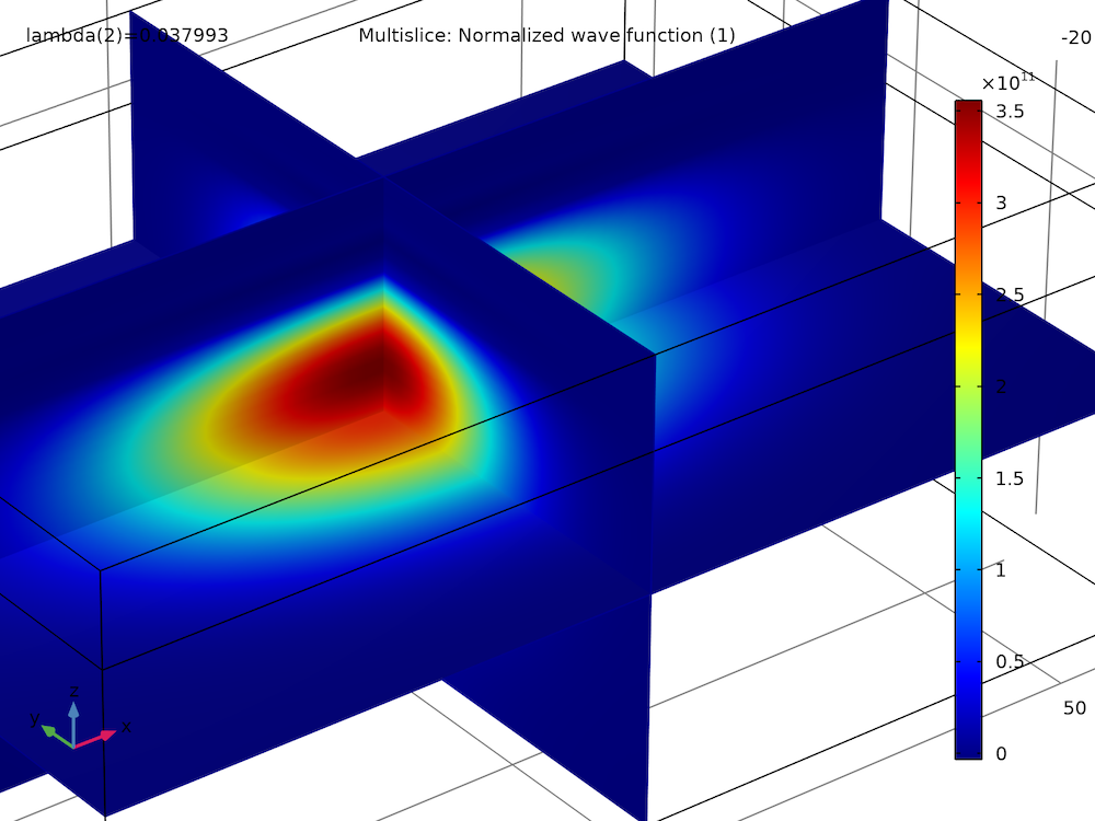
|
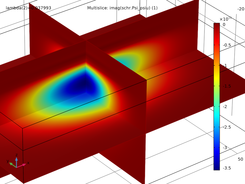
|
| First excited state, real part | First excited state, imaginary part |
The spin-down wave function components also have this trend among themselves and as compared to the spin-up components.
To understand this observation, we evaluate the wave function components near the peak density point:
| Eigenvalue | up (1), Point: (0, 0, -2) | down (1), Point: (0, 0, -2) |
|---|---|---|
| 0.03788 | 1.000+1.000i | 1.000-1.000i |
| 0.03799 | 1.000-1.000i | 1.000+1.000i |
We find that for the ground state (the first row of the result table shown above), up to an overall scaling factor of about 3.6e11, the amplitude of the spin-up component is 1+i=(1)(1+i), and the amplitude of the spin-down component is 1-i=(-i)(1+i). Therefore, the vector formed by the two components is proportional to \left(\begin{array}{c}1\\-i\end{array}\right), which is recognized as the spin-down eigenstate of the y-spin operator S_y. This is consistent with the intuitive picture that the lower-energy state of an electron in a magnetic field has its spin magnetic moment parallel to the magnetic field, and thus the spin is antiparallel to the magnetic field.
Similarly, for the first excited state, up to an overall scaling factor of about 3.6e11, the amplitude of the spin-up component is seen to be 1-i=(1)(1-i), and the amplitude of the spin-down component is 1+i=(+i)(1-i). Therefore, the vector formed by the two components is proportional to \left(\begin{array}{c}1\\+i\end{array}\right), which is recognized as the spin-up eigenstate of the y-spin operator S_y. This is consistent with the intuitive picture that the higher-energy state of an electron in a magnetic field has its spin magnetic moment antiparallel to the magnetic field, and thus the spin is parallel to the magnetic field.
This observation can be further confirmed by comparing the energy difference between the two computed eigenstates, with the expected energy difference between a spin-up and a spin-down electron in a uniform magnetic field (2\, \mu_B B), using global evaluations:
| Eigenvalue | Computed Energy Difference (meV) | Expected Energy Difference (meV) |
|---|---|---|
| 0.03788 | 0.1158 | 0.1158 |
We see a very good agreement of the computed and expected energy difference between the first two eigenstates — both evaluate to the same value of 0.116 meV.
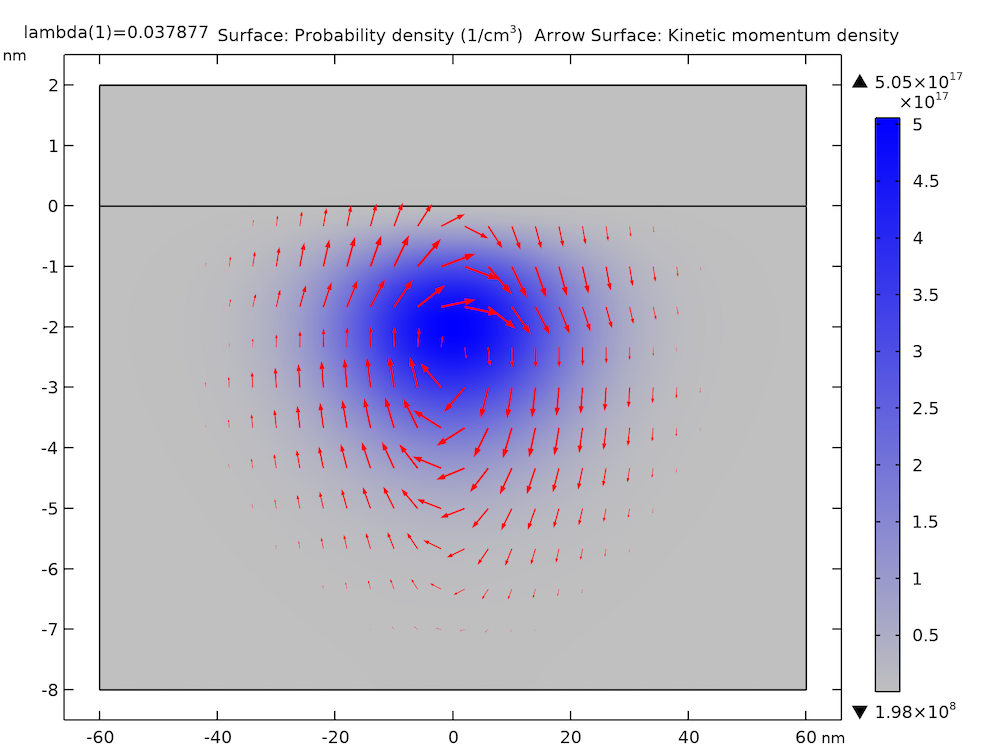
Probability Density and Kinetic Momentum Density
The plot below shows the probability density (blue-gray gradient) and kinetic momentum density (red arrows) of the ground state on the xz-plane. It compares well with Supplementary Figure 1 in the paper.
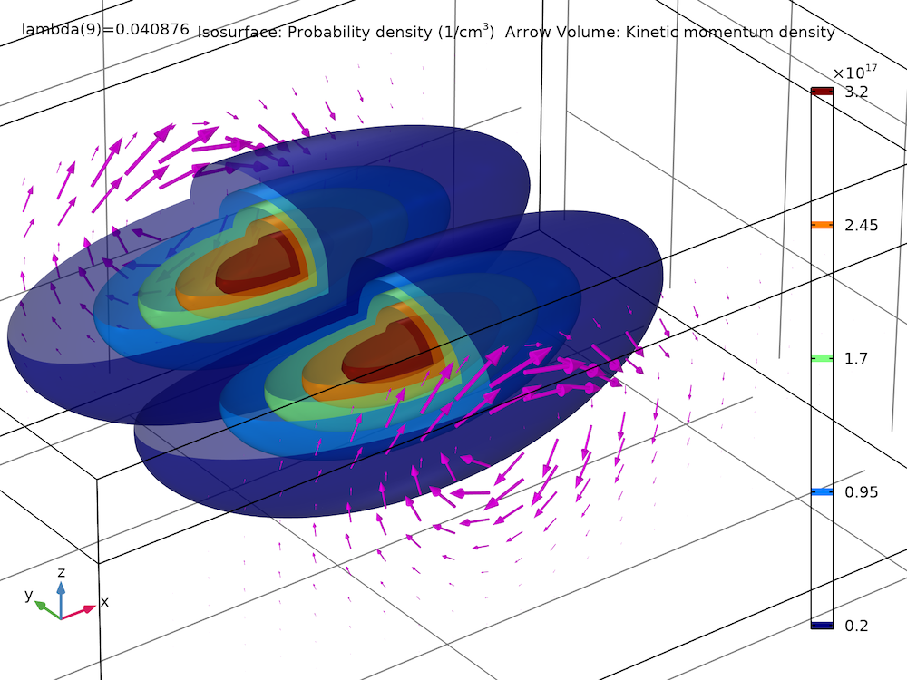
The plot below shows the probability density (isosurfaces) and kinetic momentum density (arrows) of the eighth excited state for the model thumbnail. The isosurfaces of the probability density are made partially transparent using the Transparency subnode, available as of COMSOL Multiphysics version 5.6.
Now It’s Your Turn…
In this post and the previous blog post on the k • p method for a strained wurtzite GaN band structure, we have discussed the functionalities of the Schrödinger Equation physics interface for multicomponent wave functions. We would love to hear how you use them for your simulation work.
Try modeling a silicon quantum dot in a uniform magnetic field by clicking the button below, which will take you to the Application Gallery, where you can download the MPH file.
Reference
- R.M. Jock et al., “A silicon metal-oxide-semiconductor electron spin-orbit qubit,” Nature Communications, 9:1768, 2018.


Comments (1)
SME Coils
May 7, 2021Thank you very much for the information you shared.