
There are several techniques out there for saving memory when solving a model. One involves splitting it into separate sections and solving these individually, instead of the entire model at once. If you want to map data from one COMSOL Multiphysics® solution to the next using MATLAB® scripting, you can do so by connecting the two software programs via LiveLink™ for MATLAB®.
One Method for Dividing and Conquering Your Model
To save memory, you can partition a large model into separate consecutive sections and then map the solution of each part to the input value of each successive part in series. When considering this technique, the most important thing to think about is your simulation’s component couplings, i.e. the degree of information the components have or use from one another.
There are a few methods available for using solutions as starting point values in COMSOL Multiphysics®. However, if you have a model that is too large to be solved in one block and the errors that are introduced by the partitioning are acceptable, you can use LiveLink™ for MATLAB® to integrate a model .mph file with MATLAB®.
Mapping Solutions to Boundary Conditions between Domains
To show you how to use LiveLink™ for MATLAB® to serve this purpose, we have a Pseudo-Periodic Model of a Heat Channel example available for download in our Model Gallery. A periodic function is a function whose values recur over a regular interval, most famously those of trigonometry (i.e. sine, cosine, etc). Pseudo-periodicity is a lesser known type of periodic response that seems periodic but never quite exactly repeats itself, such as your heartbeat or respiration rate, for example.
In the modeling example, we simulate convective heat transfer in a channel filled with water and solve the model by taking a pseudo-periodic section of the pipe and solving it repeatedly for temperature in successive sections up to the total length of the channel. We use the solution for temperature at the outlet boundary as the temperature at the inlet boundary for the following section of piping until we have solved for all the sections.
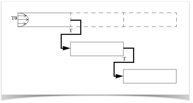
Mapping temperatures between channel sections.
Once we have set up our simulation in COMSOL Multiphysics, we can connect with MATLAB using LiveLink™ for MATLAB®. Before each step in the model, the temperature from the outlet boundary of a section is mapped to the inlet boundary of the next section using the for-loop command within MATLAB.
The number of iterations we specify will determine the number of times the pseudo-periodic section is repeatedly solved, which represents the number of successive sections that will be solved for. In this case, we are dividing the channel into six pieces so, the number of iterations would be six. After the first solution computes, an if-statement command is incorporated into the script, so that the previous solution is pulled and used for the next iteration.
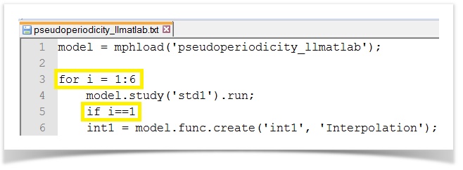
For-loop and if-statement commands in the MATLAB script.
After the model solves, we can generate a plot of the temperature distribution for each solution through the COMSOL Multiphysics wrapper function, “mphplot”. The image below shows the solution for each section of the channel, which corresponds to each of the six iterations performed.
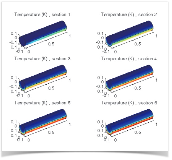
Temperature distribution along channel length, the inlet is the left boundary of section 1.
The sections can also be placed together to view the temperature distribution along the entire channel. As the water flows through, it reaches a maximum temperature of 306.5 K.
Model Download
MATLAB is a registered trademark of The MathWorks, Inc.

Comments (1)
Ahmed oudenani
January 25, 2023Dear Amelia Halliday
How can I connect comsol 6.0 to matlab?