
When creating an open-plan office, two key considerations that acoustic designers must account for are noise level and sound propagation. The COMSOL Multiphysics® software offers the tools to model an open-plan office space and run simulations to analyze its acoustics, as featured in the Acoustics of an Open-Plan Office Space tutorial model. COMSOL Multiphysics® also offers GPU support for the Acoustics Module, significantly increasing computational efficiency.
Open Floor Plans, High Noise Levels
One common complaint with open layouts is noise level. The architecture, engineering, and construction industries have a growing interest in mitigating noise issues while designing open layouts. Acoustics modeling enables engineers in these industries to simulate noise levels efficiently and optimize designs ahead of physical construction of an office space.
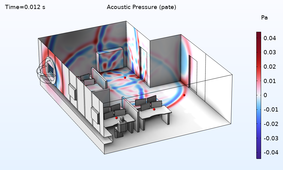
Pressure distribution depicted on the walls of a small open-plan office with a pulse emitted from a point 1.5 m above the floor.
Building a Digital Office
In the Acoustics of an Open-Plan Office Space tutorial model, the acoustics of an open-plan office space are analyzed using a wave-based approach in the time domain. An initial pulse is emitted and the room response is analyzed. Realistic frequency-dependent impedance conditions for several aspects of the room — including the ceiling, carpet, and gypsum bolts on the walls — are included using the General Local Reacting (Rational Approximation) impedance option. The Partial Fraction Fit function is then used to fit the input data. An open window is also modeled using the Absorbing Layer feature. This model is solved with the Pressure Acoustics, Time Explicit interface and uses the accelerated solver formulation, which can be run on one or more GPUs.
COMSOL Multiphysics® version 6.4 extends the existing single-GPU support to multi-GPU configurations, for accelerated simulations of pressure acoustics in the time domain, allowing speedups of 25x and more compared to using CPUs. To run the model, 12 gigabytes (GB) of GPU memory are required and a NVIDIA® GPU are required. The version used here is 6.4 build 343.
Solving 20 periods of the 500-Hz carrier signal (mesh resolution up to 750 Hz) on a CPU with 12 cores takes about 10 hours (hardware dependent), whereas solving the same 20 periods on two GPUs takes 9 minutes. This initial analysis gives the propagation for the first 25 ms, and is useful for visualizing the initial propagation of the pulse.
Pressure distribution is depicted in red and blue on the walls of an open-plan office space. A pulse is emitted from a point 1.5 meters above the floor, near the bookshelf along the back wall. Frequency-dependent impedance conditions are used to describe the boundaries.
The model includes several impedance conditions, which use frequency-dependent data. The complex-valued impedance data is generated using the Acoustic Treatment Boundary Calculator, a simulation app for analyzing dispersion. The app can compute several properties or boundary properties that can then be used in room acoustics simulations. The data for various aspects of the model, such as the carpet, ceiling, and gypsum bolts on the walls, is computed using the app.
The open window along the left wall is included in the model to highlight the use of absolving layers together with the GPU. You can add half a sphere with absolving layers on the outside of the window to model the open window in this space.
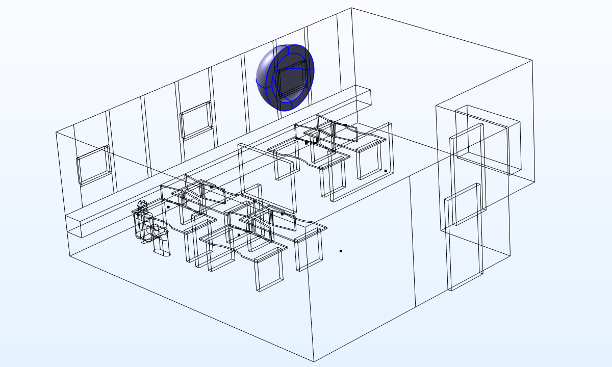 A half sphere with the absolving layers, added onto the outside of the open window.
Studying Microphone Points
This open-plan office space acoustics model solves for 46 million degrees of freedom (46 \cdot 10^6 DOFs) in two studies. In study one, the model solves for 20 periods of the 500-Hz carrier signal, storing the solution twice per period on all boundaries. This study takes 9 minutes to solve on two GPUs (15 minutes on one GPU) and looks at the sound field in the beginning of the propagation of the pulse. To analyze the impulse response of the system, a second study is run, where the solution is only stored in the selected microphone points.
In study two, the model solves for a duration of 0.4 s (300 periods), storing the solution with a higher resolution 30 times per period only, on selected receiver positions. This study takes 2 hours and 56 minutes to solve on two GPUs. The signal is again received at the microphones (see image below). By using the impulse response plots, the level decay curves for 1/3 octave bands can be computed and analyzed. This enables you to compute room acoustics metrics that would typically be done using ray acoustics, with a more accurate full-wave method (more accurate in the low to medium frequency limit).
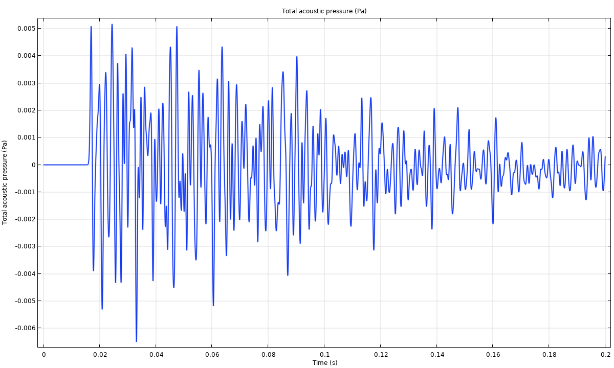 Impulse response for the microphone position closest to the manikin.
Extending the simulation time from 20 periods to 300 periods would suggest that it takes 2 hours and 15 minutes to solve study two, instead of the 2 hours and 55 minutes that it takes. This is due to a small overhead as a result of storing the solution more often. Storing the solution 30 times per period, compared to 2 times per period, creates a relatively small overhead and time difference, as well as some additional communication between the GPU and CPU.
 The locations of the microphone points throughout the open-plan office space.
The level decay curves (for three 1/3 octave bands) computed for the microphone location closest to the manikin (see figure above) is depicted in the figure below. For the three bands the T20 reverberation time is about 0.65 s.
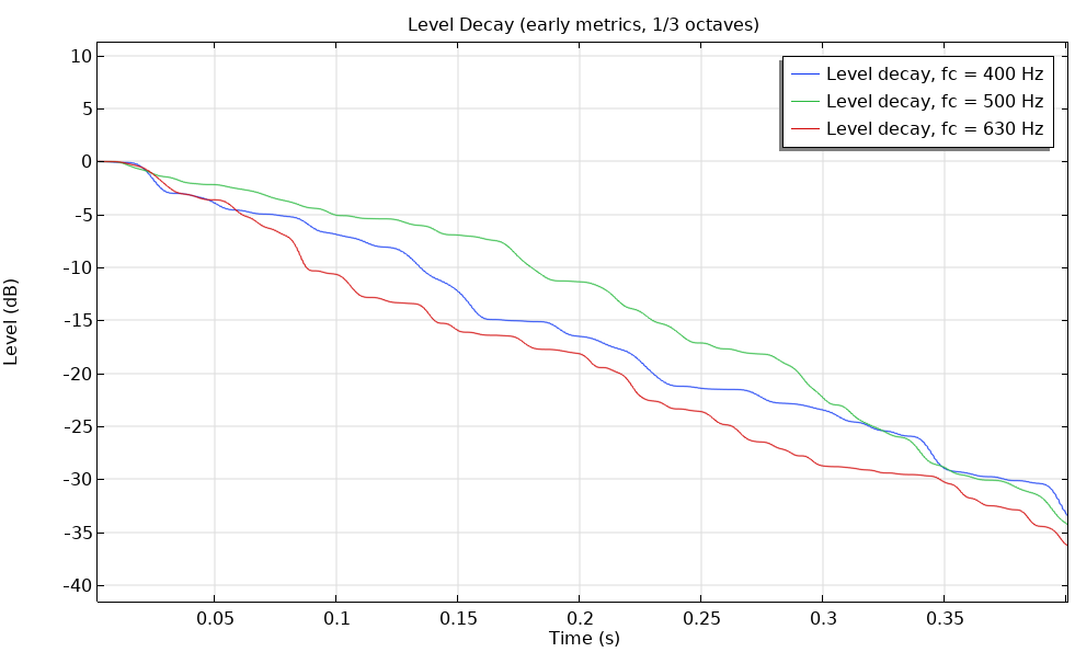 Level decay curves for the three 1/3 octave bands centered at 500 Hz.
Fitting the Impedance Data
In some sets, the Partial Fraction Fit function is used for rational approximations instead of nominal approximations. In the Frequency Domain Data graph shown below, there is a high number of points in the graph and both real and complex values of the admittance. The data needs to be fit using an approximation, and the approximation data is done with a partial fraction fitting. This equation approximates the data with a sum of fractions.
When the frequency-domain data is approximated with this formula, there is an analytical inverse Fourier transform of the data. With the Fourier transform, the data can then be used in the time domain in a more practical way. This translates into a lumped system or a system of memory ODEs that can be solved together with domain equations. This setup is handled automatically in COMSOL®.
After the data has been fitted, the fitting parameters can be used in the time domain to model frequency-dependent properties, for example, an impedance condition or porous materials.
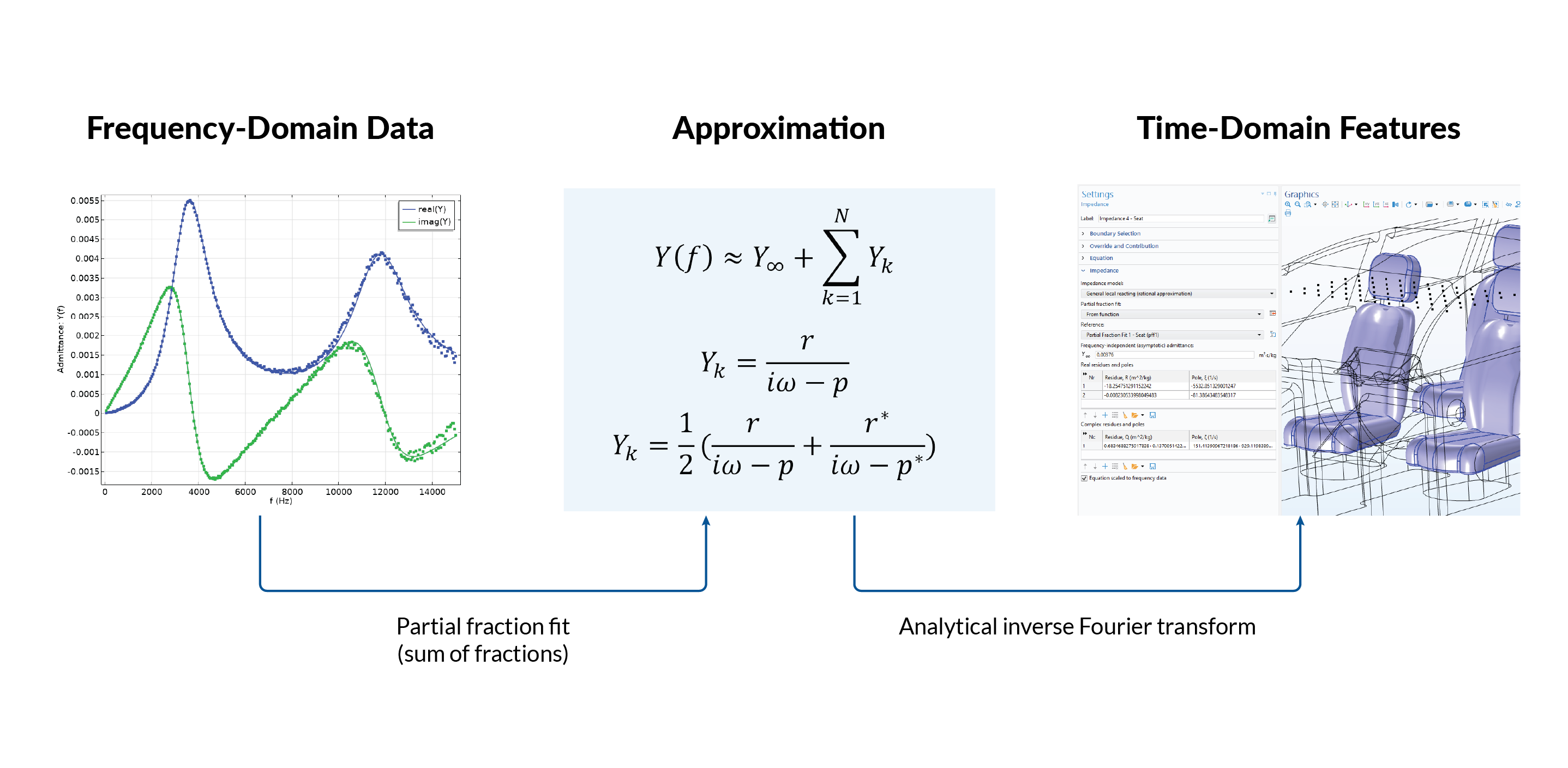 The frequency-domain data is approximated with this formula, creating an analytical inverse Fourier transform of the data.
What’s Next?
As the trend of open-plan office spaces continues to grow, mitigating noise levels will be a top concern in layout design. Try out the Acoustics of an Open-Plan Office Space tutorial model or Acoustic Treatment Boundary Calculator demo app yourself.
Further Reading
If you’d like to learn about a real-world use of modeling and simulation for improving the acoustical conditions of a workplace, you can check out our article, featuring Swiss consultancy Zeugin Bauberatungen, “Harmonizing Sound and Style in Open-Plan Offices”.


Comments (0)