When working with imported data that varies over space, we often face the challenge of determining what level of mesh refinement is needed to accurately resolve the input data and how it affects the solution to our multiphysics problem. We can use adaptive mesh refinement in these cases to refine the mesh based upon the model results. As it turns out, we can also use adaptive mesh refinement to refine based upon the input data. Let’s learn more!
Modeling a Nonuniform Heat Load
Consider the problem shown below of a plate of material that is heated from above with a spatially varying heat load that comes from an external data file and has some distinct, but quite nonuniform, structure to it.
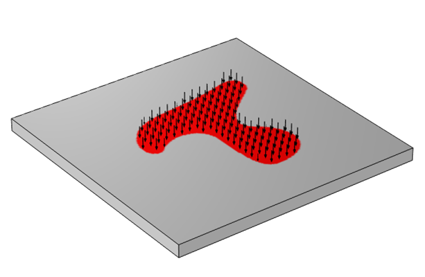
Visualization of a nonuniform applied heat load that is read in from an external data file.
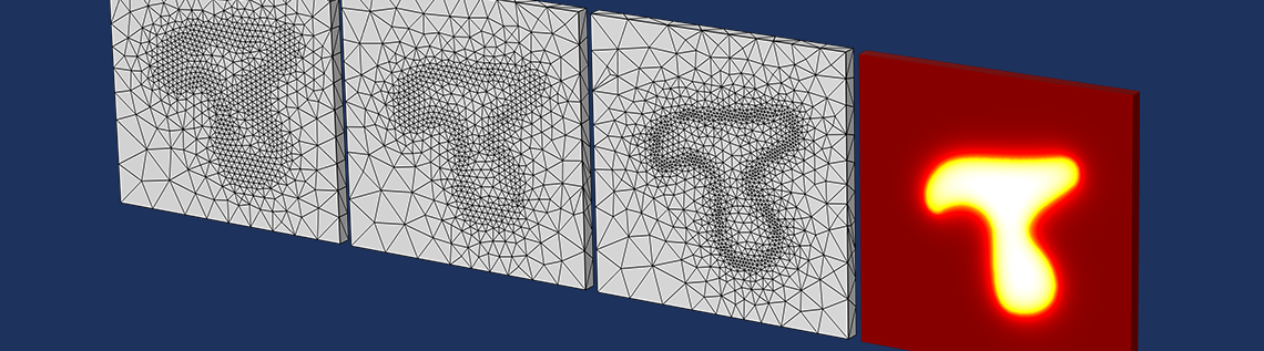
This actually doesn’t present a problem for the COMSOL Multiphysics® software at all. We can simply use adaptive mesh refinement and the COMSOL® software will automatically refine the mesh several times, as specified by the user, to give us a more accurate solution to the problem. Several iterations of this algorithm are plotted below.
Results showing the mesh (top view) when using adaptive mesh refinement. Starting with a uniform mesh, the software adapts the element size to accurately resolve the variations in the solution due to the spatially varying applied heat load. This reproduces the spatial variation of the applied load, but it takes several iterations for this structure to become apparent.
What we can observe is that the adaptive mesh refinement algorithm started from the default mesh, which has no knowledge of the shape of the applied heat loads. Only after several iterations does the algorithm really start to identify the distribution of the load very well, and there is some computational expense to these initial iterations.
What if there was a better way? What if we could tell the software that we want to start with a mesh that is already adapted to the shape of the experimental data? We still want to perform adaptive mesh refinement, of course, but we want to start this refinement process from a more reasonable initial mesh.
It turns out that this is very easy to do by implementing a Helmholtz filter over just the imported data and adapting the mesh on that. We’ve already introduced the concept and implementation and some benefits of the Helmholtz filter in a previous blog post. Now let’s look at another capability that it gives us.
Implementing Adaptive Mesh Refinement and Data Filtering
We can implement a Helmholtz filter equation on just the top surface of our model, with quite a small filter radius (think of this radius as akin to the spatial resolution of the input data) and solve it on a quite coarse mesh, just on the surface. The Helmholtz filter equation itself is linear, so it can be solved on any mesh, and the adaptive mesh algorithm will be able to identify where this mesh needs to be refined. We just need to make a few small tweaks to the solver and mesh settings.
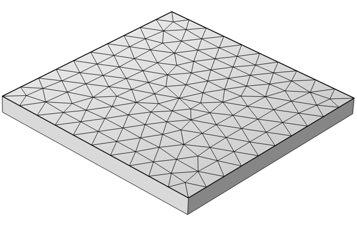
The mesh that is used to start the adaptive mesh refinement is applied to just the top surface of the part.
Within the Stationary step, where we solve for the Helmholtz filter, there is just one required change. The Geometry Entity Selection for Adaption must be modified so that the adaptation is performed only over the regions where the filter is defined (in this case, just a single boundary). You can also optionally increase the Maximum number of adaptations and experiment with the adaptation method, especially the General Modification and Rebuild Mesh options.
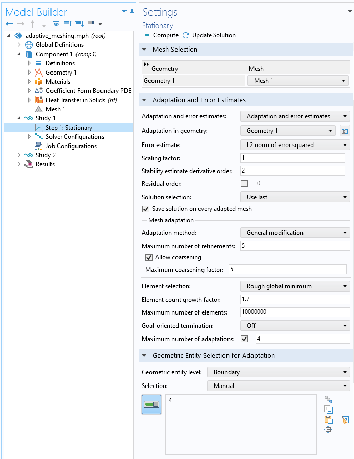
Settings that define the adaptive mesh refinement of the boundary.
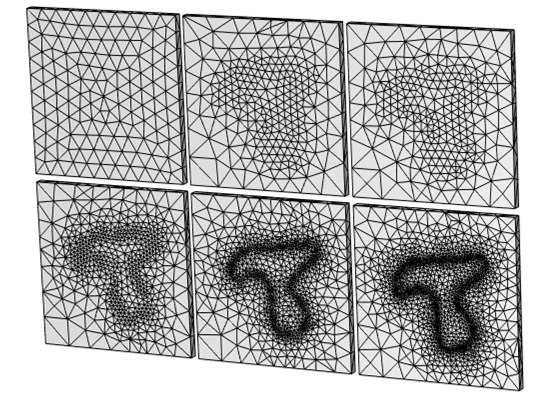
All other settings can be left at the defaults. When solving, you’ll get a sequence of meshes that adapt solely based upon the filter solution on the boundary, as shown below. There may be some messages in the solver that there is no mesh within the volume, but this is desired: We want to adapt only the mesh on the surface, not do any remeshing of the volume — yet.
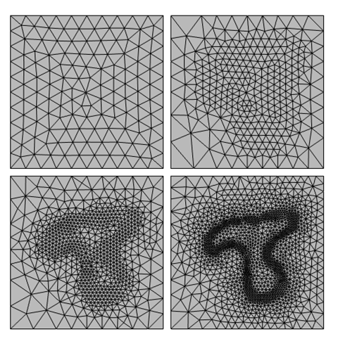
The sequence of the first four meshes generated by the adaptive mesh refinement algorithm. These exist solely on the top boundary.
Using the Adapted Mesh to Solve the Problem
Next, we want to use one of the adapted surface meshes within the definition of the volumetric mesh used to solve the heat transfer problem. All we need to do is add another mesh, of the type User-Defined, and add a Reference feature within it, immediately after the global Size feature that is always present in a mesh sequence. After that, we add a Free Tetrahedral feature, and we have a complete mesh that can be used to solve the heat transfer problem.
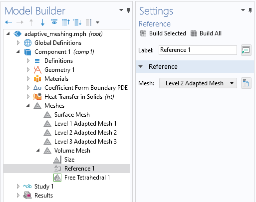
Building a new volumetric mesh based upon the results of one of the previous adaptively refined boundary meshes.
In fact, we could even perform additional mesh refinement, working forward from this mesh. The advantage is that we’ve already started with a mesh that is quite well adapted to the applied loads. So, for this problem, we don’t need to do very much adaptive mesh refinement of the thermal solution.
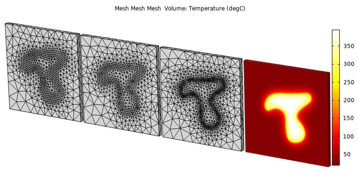
Starting from the mesh refined based upon the input data, we don’t need to refine the mesh as many times to get confidence in the model solution.
We can see here that there’s a clear computational benefit in this case. Any time that you are reading in experimental data that varies quite sharply in space, it will be worth investigating this technique, as it can save significant computational effort. If, on the other hand, the data is relatively smooth, without sharp transitions, then this technique is not as strongly motivated.
It is also worth mentioning that in this case we focused on a 2D planar surface, so you could also use the approach of treating the heat distribution as an image file, and convert that image to a set of curves, which can be used within any 2D workplane. That approach, however, is only applicable for 2D planar surfaces, while the approach presented here can also work on curved surfaces and even volumes.
Try It Yourself
Click the button below to access the files associated with the model example discussed here:


Comments (0)