The fast Fourier transform (FFT) is a useful and powerful numerical method. The latest release of the COMSOL Multiphysics® software, version 6.0, introduced a new feature relating to this method: the Spatial FFT feature. In this blog post, we will discuss how to use this new feature for optics and show application examples.
Terminology and Definition
First, let’s make the terminology and definition clear. There are three terms to distinguish: the Fourier transform (FT), discrete Fourier transform (DFT), and FFT. The FT of a function u is defined as
where x and \xi are variables in physical space and Fourier space, respectively. The variable \xi is referred to as the frequency when the physical space variable is time t. In optics, \xi is referred to as the spatial frequency, which is typically scaled with the wavelength and the focal length (we will discuss this later), whereas x is the physical space coordinate used to describe the location in the vicinity of the optical structure of interest.
In previous blog posts, “How to Implement the Fourier Transformation in COMSOL Multiphysics” and “How to Implement the Fourier Transformation from Computed Solutions”, we discussed how to carry out the FT in COMSOL®. We can use a numerical technique that performs the Fourier transformation formula by direct numerical integration based on Simpson’s rule. We may call it “the FT by numerical integration” later in this blog post.
The DFT is the discrete version of the FT, which carries out operations on a discrete set of points. In COMSOL®, it’s defined as
The FFT is an efficient algorithm that computes the DFT.
Note that these definitions for the FT and DFT are the most general definitions, but the sign convention is not consistent with COMSOL’s sign convention for the wave formulation, which is \exp(i(\omega t- {\mathbf k}\cdot {\mathbf x})). We knowingly use this standard definition with care when we use it for Fraunhofer and Fresnel diffraction formulas. The inconsistency doesn’t affect the stationary solutions.
How to Use the Spatial FFT Feature
Let’s demonstrate how to use the new Spatial FFT feature in COMSOL® for optics. The FFT feature can be set up and carried out using steps 1 and 2, respectively:
- Step 1: Prepare the dataset
- Add a Spatial FFT dataset by right-clicking Datasets → More Datasets (this defines the Fourier space)
- Select an appropriate source dataset as the physical space, which is then transformed
- Set Spatial resolution to Manual
- Set Sampling resolution to an appropriate number
- Choose Use zero padding from Spatial layout and set x padding to an appropriate number
- Choose Frequency in Fourier space variables
- Uncheck Mask DC
- Step 2: Plot using the
fft()operator- Adjust the spatial frequency scaling for the x-axis data in the plot settings
Rectangular Function Example
The rectangular function is one of the most frequently used functions in optics because it represents a hard aperture. When there is a hard aperture, the FT of the rectangular function is always involved. The Fourier transform of the rectangular function can be easily calculated by hand and is known as:
\begin{cases}
0 & |x|>a/2 \\
1 & |x|\le a/2
\end{cases}
where \mathcal F stands for the Fourier transformation operator, a is a constant, and {\rm sinc}(x) = \sin x/x is the sinc function.
Let’s take a look at how this FT is calculated with the new Spatial FFT feature in COMSOL®.

An example of the dataset settings for the rectangular function (left) and its FT (right).
The rectangular function is a built-in function under Definition > Functions. If you press the Create Plot button, a new dataset for the function is automatically created under the Datasets node under Results. The range and resolution are also automatically set by default. When performing the FFT, it’s important to control these parameters yourself. The Fourier space resolution is determined by the reciprocal of the physical space range and the zero padding to the physical space data. The Fourier space range is determined by the physical space range and the Fourier space sampling number. The magnitude of the FFT results varies by the physical space range and the Fourier space sampling number. The following table is the summary of the FFT parameter expressions, including parameter values that correspond to the FFT settings shown in the previous image.
| Parameters | Expression | Example Values |
|---|---|---|
| Physical Total Range | X_0 |
|
| Fourier Space Sampling Number | N_x |
|
| Zero Padding | N_z |
|
| Fourier Space Total Range | N_x/X_0 |
|
| Fourier Space Resolution | \frac{N_x}{X_0} \cdot \frac{1}{N_x+2N_z} |
|
| FT Normalization Factor | X_0/N_x |
|
With the abovementioned settings, the following plots are the rectangular function, rect1(x), and the absolute value of its FT, abs(fft(rect1(x)), is computed by the FFT feature. The Fourier space total range is N_x/X_0 = 16/2 = 8, i.e., from -4 to 4. You can see that the total number of sampling points in the Fourier space is N_x+2N_z = 32.
Why 2N_z? That’s because, in zero padding, N_z zeros are added to both sides of the physical space data. The Fourier space resolution is 8/32 = 0.25. Without normalization, the FFT operation results in the factor of N_x/X_0. So, we need to multiply the results by X_0/N_x to get a unit peak value. Later on, we will use the FFT for various formulas, each having a different multiplication constant. Because of this, we have to normalize the FFT result to unity.

Rectangular function with a = 1 and the absolute value of its FT, as determined by the FFT and the settings shown earlier.
In this example, the sampling number was intentionally set to a low number so that you can reference the preceding formulas. Still, we can see that the FT, {\rm sinc}(\pi \xi), is calculated with a good approximation. With more appropriate parameters (X_0 = 3, N_x = 128, and N_z = 512, for example) we get the following results, which are perfect. The result for the FT by numerical integration is overlaid for comparison. Of course, the two methods should match!

A comparison of the rectangular function with a = 1; the absolute value of its FT, as determined by FFT, which has a higher resolution; and the FT by numerical integration.
Fourier Transformation in Optics
So far, we have learned how to set up and use the Spatial FFT feature for a rectangular function, which is a 1D analytical function. Now let’s use it for some practical application examples in optics.
In optics, the time-frequency Fourier transformation, which relates a temporal signal of the electric field of light to its spectra (frequencies or wavelengths), may be more well known. The spatial Fourier transformation is used in various propagation (transformation) methods for an electric field traveling from one plane to another. In this case, the spatial Fourier transformation relates the spatial shape of an electric field in a plane to the shape (called the spatial frequency) in the other plane. Let’s consider a scalar electric field or a component of a vector electric field that is incident on a disturbance in a plane, such as an aperture or a lens, and then arrives at another plane, such as a focal plane or image plane, as shown in the following figure:
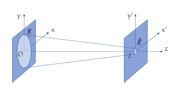
Coordinate system for the propagation (transformation) method in optics.
Let’s denote the electric field in a plane after the disturbance E(x,y,0). Then, the electric field in another plane, \hat{E}(x’,y’,L), is calculated using one of the four propagation methods, depending on the purpose. The following table summarizes the four methods. The formulas are represented by a simple notation for the Fourier transform, \mathcal{F}[\cdot], up to a trivial phase function.
| Theory | Formula (Simple Notation) | Application |
|---|---|---|
| 1. Fraunhofer diffraction theory | \hat{E}(x’) = {\mathcal F}[E(x)] |
|
| 2. Fresnel diffraction theory | \hat{E}(x’) = {\mathcal F}[E(x)\exp(-ikx^2/(2L))] |
|
| 3. Angular spectrum method*** | \hat{E}(x’) = {\mathcal F}^{-1}[{\mathcal F}[E(x)]\exp(ik\sqrt{1-\alpha^2})] |
|
| 4. Partial coherence theory (Schell model)**** | I_{pc}(x’,L) = {\mathcal F}^{-1}[{\mathcal F}[I_c(x)] {\mathcal F}[\gamma(x)]^\ast ] |
|
Footnote:
* Fraunhofer diffraction condition
** Fresnel diffraction condition
*** \alpha is the direction cosine
**** I_{pc} is the partially coherent intensity, I_c is the coherent intensity, and \gamma is the mutual coherence function
Fraunhofer Diffraction
The Fraunhofer diffraction formula is used to calculate the far field that is diffracted from an object when the Fraunhofer condition is met.
The following is the full formula:
(x’,y’,L) = \frac{e^{i k L}}{i \lambda L} \iint_{-\infty}^{\infty}E(x,y,0) e^{-i 2\pi (x’ x+y’ y) / (\lambda L)}dxdy
This formula is used for calculating the far field of apertures, gratings, and the field in the focal plane of Fourier optics (Ref. 1). The object is a square aperture with a uniform illumination. The electric field at the exit plane of the aperture is a 2D rectangular function and the far field is calculated by the FFT. This forms a diffraction pattern, which may be a familiar sight: it is similar to how lit street lights look when viewing them from behind a mesh curtain. Note that you need to scale the x-axis data in the plot by the factor of \lambda L since the spatial frequency is scaled as f=x’/\lambda L. Computing a 2D FT using the FT by numerical integration takes a long time but the FFT can do the job very quickly.
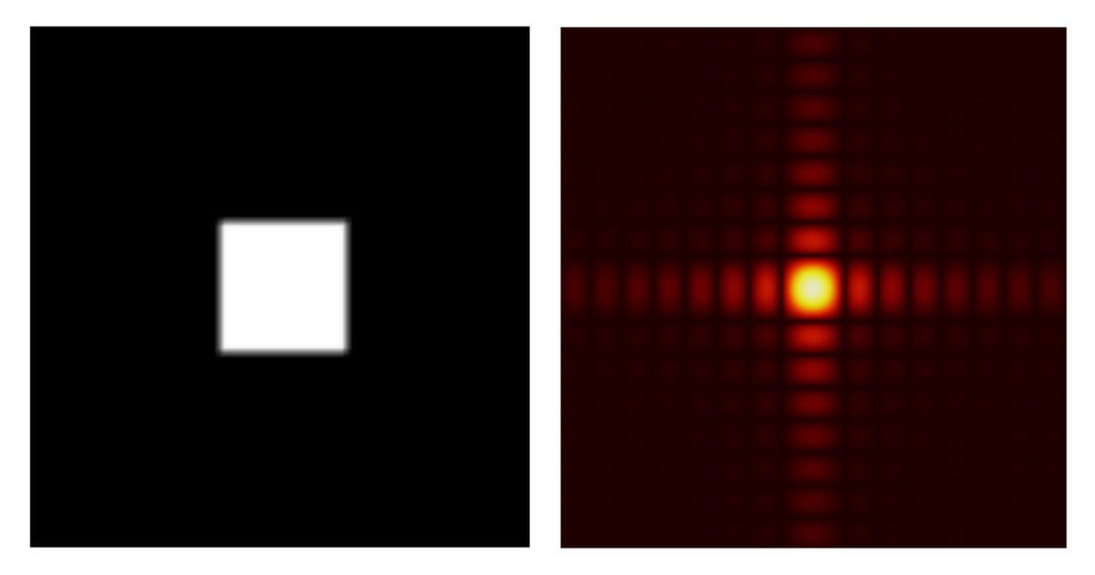
A square aperture (left) and its diffraction pattern (right).
The settings for simulating a square aperture are quite easy:
Fresnel Diffraction
The second application, the Fresnel diffraction formula, can be used for calculating the far field as well as the field near the disturbance. The full formula for this approximation is:
Note that the x-axis data needs to be scaled by the factor of \lambda L. This application is implemented in the Fresnel Lens model, in which the Wave Optics, Frequency Domain interface was used for computing the electric field inside the lens. The Fresnel diffraction formula was then used for calculating the field in the focal plane by the FT by numerical integration. As shown in the figure below, the FFT feature can be used in this model and give the same result as the FT by numerical integration.
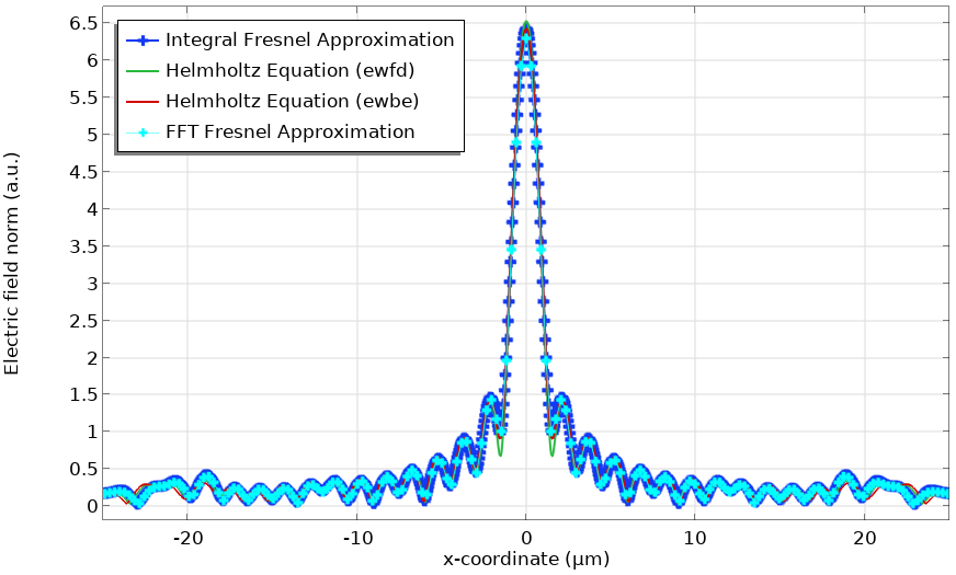
Electric field norm in the focal plane of the Fresnel Lens model. The FFT feature is used for computing the Fresnel diffraction formula and is compared with other methods.
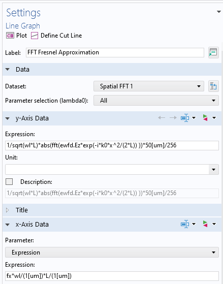
Postprocessing settings for the FFT feature for the Fresnel diffraction formula. Note that the y-axis data is normalized and the x-axis data is scaled.
Angular Spectrum Method
The third application, the angular spectrum method, is a bit tricky to implement because it requires using the FT twice, as you can see in the full formula:
where
and \alpha and \beta are the direction cosine.
In the previously mentioned blog posts, we presented how to simulate large optics; i.e., You can use either the Wave Optics, Frequency Domain interface for calculating a small domain around an optical component and then use the Fraunhofer or Fresnel diffraction formula, or use the Beam Envelopes interface for simulating the entire domain. However, these two methods only work for slow (low-NA) lenses, as fast (high-NA) lenses require a lot of mesh elements, which the Fraunhofer and Fresnel formulas cannot give good approximations for. The wave vectors are too steep for the Beam Envelopes interface to mesh the computational domain.
The only way to simulate large high-NA lenses is to use the angular spectrum method (ASM). This is a propagation method that belongs to the same type of numerical method as the Fraunhofer and Fresnel diffraction formulas. Once the field in one plane is known, the field in another plane can be calculated. The ASM is rigorous because it satisfies the Helmholtz equation. This method could be combined with the Wave Optics Module to compute the field in a certain domain, and then the ASM could be used to propagate the field to a farther plane.
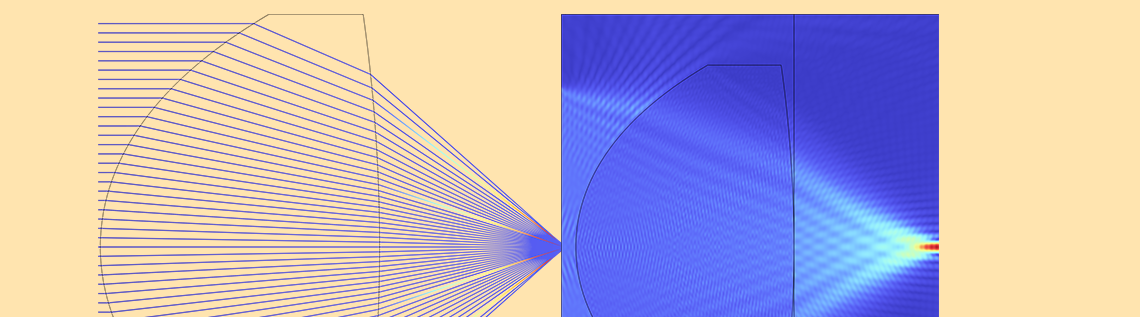
Below is an example of a high-NA lens (NA = 0.66), which is much faster than the DVD pickup lens. The radius of the lens is 16 μm and the back focal length (distance between the second surface of the lens and the focal plane) is 10 μm. The lens is optimized to be diffraction-limited for the wavelength of 0.66 μm using the Geometrical Optics interface in combination with the Optimization Module. The lens was intentionally designed to be small so that the Wave Optics, Frequency Domain interface can compute the rigorous solution for comparison. We will demonstrate how to propagate the field from the exit surface of this lens to the focal plane using ASM.
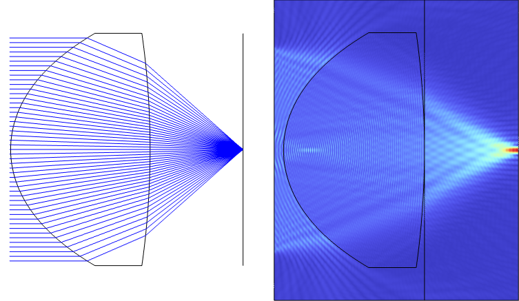
An NA = 0.66 lens designed using the Ray Optics Module and the Optimization Module (left). A full-wave simulation of the lens simulated using the Wave Optics, Frequency Domain interface (right). Note the line representing the lens exit plane, from which the field is propagated to the rightmost edge, i.e., the focal plane.

Spot profile of the NA = 0.66 lens model comparing the Fresnel diffraction formula; the rigorous solution by the Wave Optics, Frequency Domain interface; and ASM. Note that the Fresnel diffraction formula is no longer accurate for this lens. (The spot profile is shown at 11 μm instead of 10 μm for better comparison.)
To perform the FT twice, we need to store the first FT in a dataset. This is because the fft() operator is merely a postprocessing operator, not a general operator, such as the integrate operator, which can be used in physics settings. For now, with the current version of COMSOL Multiphysics (until the fft() operator is promoted to a general operator in a future version), we still need to use the FT by numerical integration in the physics setting for the first FT and then use the fft() operator for the second FT in the postprocessing. The Boundary ODEs and DAEs interface with the Distributed ODE node is defined on the lens exit plane, on which the first FT is carried out using the FT by numerical integration and the result is stored as a function, u, as shown in the following image:

Screenshot of the settings for the Boundary ODEs and DAEs for the first FT in the ASM. Note that we normalized the Fourier space by the lens radius, D/2, for an appropriate scaling.
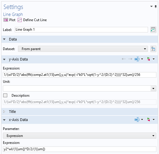
Screenshot of the settings for the second FT in ASM in postprocessing. Note that the direction cosine, a, is represented in the y-axis data by the normalized y-coordinate, \alpha = y/(D/2), and the normalization factor 1/wl in the x-axis data comes from the differential of the variable d(\alpha/\lambda) for the second FT. Also note that the spatial frequency name y2 is arbitrarily chosen in the Spatial FFT dataset.
It’s worth mentioning that the second FT is actually the inverse FT, but there isn’t a difference between the absolute value of the FT and the inverse FT up to the constant. Having seen that ASM gave an accurate result as the Helmholtz solution, we can use this technique for other high-NA lens systems, e.g., large high-NA Fresnel lenses.
Concluding Remarks
We have seen the basics of how to set up the new Spatial FFT feature and examples of how it can be used in some important applications in optics. We will talk about the fourth application, the partially coherent beam calculation (with the formulation being the same as what was used for the third application here), in the next blog post in this series.
References
- J. W. Goodman, Introduction to Fourier Optics, 3rd ed., Roberts and Company Publishers, 2005.
- M. Born and E. Wolf, Principles of Optics, 7th ed., McGraw Hill, 1968.
- A. C. Schell, “A technique for the determination of the radiation pattern of a partially coherent aperture,” IEEE Trans. Antennas Propag., vol. 15, no. 1, pp. 187–188, 1967.


Comments (2)
Charles-Antoine CLAVEAU
October 2, 2022Dear Dr. Mizuyama,
Thank you so much for this new blog post, which like the previous ones, is very instructive and shows how to make the most of COMSOL thanks to the synergy between its different modules.
I recently started using COMSOL for optical simulations. I was wondering if it was possible in COMSOL, in the same vein as the methods discussed above, to compute the PSF in the image plane of an optical system as follows:
1- first determine by *ray tracing* the wavefront in the exit pupil of the system,
2- then compute the diffraction pattern (=PSF) by propagating in the image plane this wavefront for example using the Fresnel (or Fraunhofer) diffraction formula,
provided of course that the strict conditions of validity of this technique are specified and met.
Your comments would be very helpful.
Thank you,
Charles-Antoine Claveau.
Yosuke Mizuyama
October 11, 2022 COMSOL EmployeeDear Charles-Antoine,
Sorry for the delay and thank you for reading my blog and for posting your valuable suggestion.
Yes, it is theoretically possible and we may have that feature in the future version of our Ray Optics module.
At the moment, writing a Java method in the Application Builder (programming environment) is the only way to do it if you dare.
Best regards,
Yosuke