
Guest bloggers André Gugele Steckel and Thomas Bisgaard discuss using traditional model-order-reduction techniques and the surrogate modeling techniques in the COMSOL Multiphysics® software for efficiently designing battery systems.
Lifetime predictions are paramount when designing battery systems, large and small. In this blog post, we present a method for performing these investigations efficiently and quickly with simulation by using new reduced-order models. This method is a paradigm shift from the traditional build-and-test method or using generalized design principles, which can be expensive, slow, and imprecise when trying to design systems that are to last decades. In the scope of the new method, the COMSOL Multiphysics® software shines bright with its multiphysics modeling capabilities and, very importantly for this showcase, its implementation of surrogate modeling for model order reduction.
Introduction
Battery Market Growth
Sales of electric cars surpassed 10 million in 2022, largely contributing to the 65% increase in demand for automotive lithium-ion (Li-ion) batteries that same year (Ref. 1). The use of batteries for large-scale energy storage is also gaining more interest because of more consistent scale-up compared to traditional gravity-reliant methods like hydropower. Battery pack efficiency, longevity, and recyclability are critical design targets in the goal to meet sustainability targets, which also entails responsible use of essential raw materials such as lithium and nickel.
Why Simulation?
Simulation is an enabling tool that helps engineers reach design targets at low resource and material cost, as it reduces experimental iterations and prevents designs from having unneeded overcapacity. However, engineers are often forced to rely on potentially impairing assumptions and nonphysical parameters to bridge small-scale (single-cell electrochemistry) simulations and large-scale (battery pack) simulations. In the revolutionizing integrated approach discussed here, deep neural networks (DNNs) are used to bridge the scales in such a way that a model’s high fidelity is maintained at a low computational cost.
This approach makes it possible to calculate degradation at every point in a 3D battery pack model at full time resolution during discharge and charge cycles. For example, with these simulation tools, design engineers can incorporate realistic use patterns to optimize battery management systems (BMS) and temperature control systems as well as to improve profit by balancing capacity, lifetime, and application specifications. An overview of the model scales and features can be seen in Figure 1.
Methodology
The methodology presented here is for multiscale and multiphysics modeling of batteries. The approach allows for modeling down to the finer details and using those results to expand the model to the whole battery pack of a car. This multiscale modeling spans from detailed electrochemical transport of lithium between the anode and cathode — including diffusion into storage particles — to system-level modeling of a full battery and multiple interconnected batteries in a pack.
We have used a combination of traditional model-order-reduction techniques and the surrogate modeling techniques in COMSOL®. By using the DNNs, we have been able to model multiscale systems in a way that we have not been able to do before.
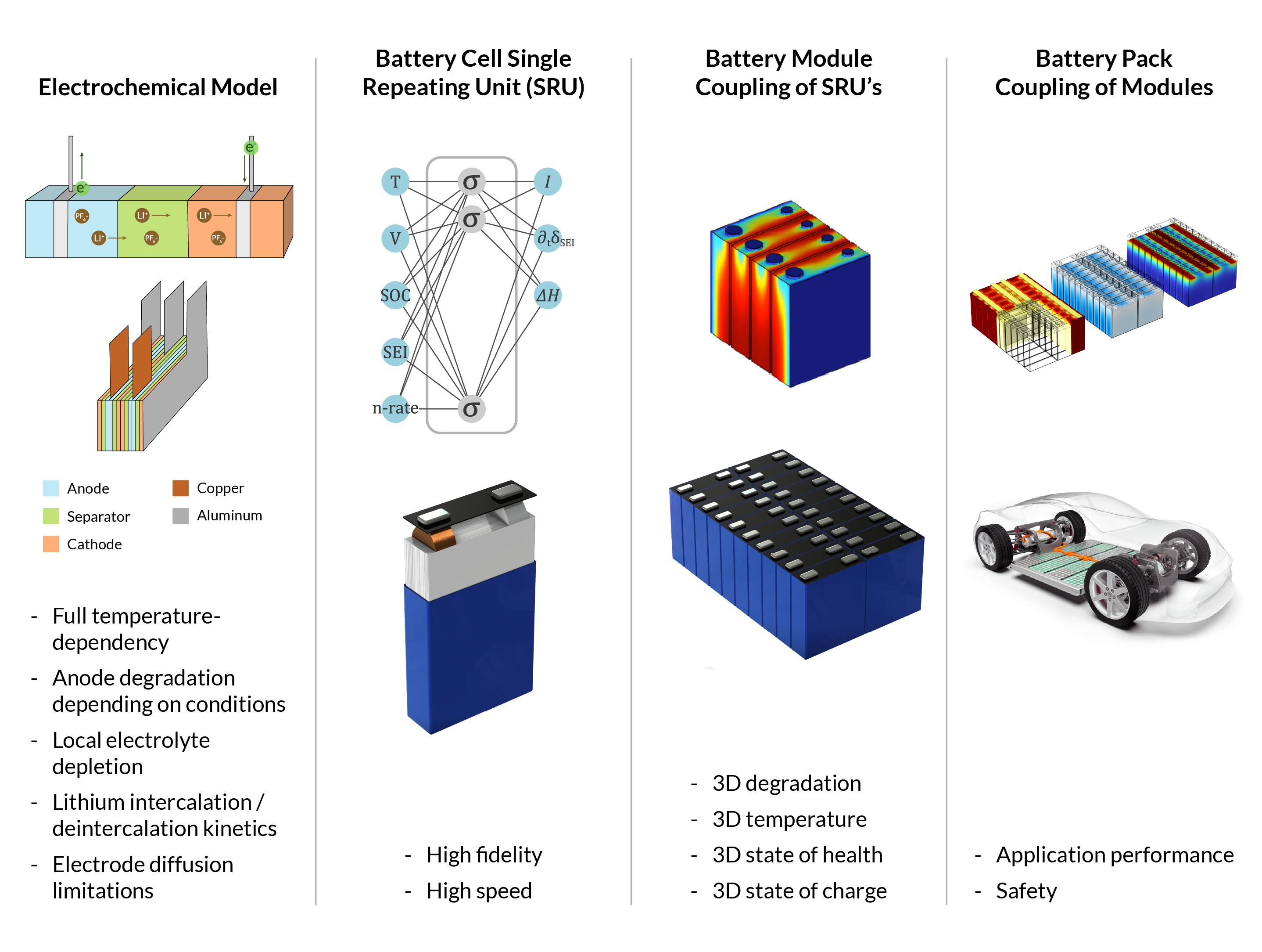
Figure 1. A multiscale approach was used for simulating battery packs, and each model scale offered different features.
Cell and Particle Scale: Battery Electrochemistry
A lithium-ion battery (LIB) consists of a repeating sequence of layers: anode, separator, cathode and current collectors on both sides (Figure 2). Each layer typically has a thickness in the range of 5 µm to 60 µm. The anode, separator, and cathode are porous structures. Within the matrices there is a liquid electrolyte. Graphite is the most common anode material. A graphite anode can be combined with a NMC (nickel–manganese–cobalt) cathode or a LFP (lithium iron phosphate) cathode. The nonconducting separator allows for electrolyte transfer. The electrolyte consists of dissociated salt (commonly LiPF6) in a solvent (commonly alkyl carbonates). Note that next-generation batteries that have different chemistries are ongoing work, including sodium-ion batteries (lithium-ion replacement) and solid-state batteries.
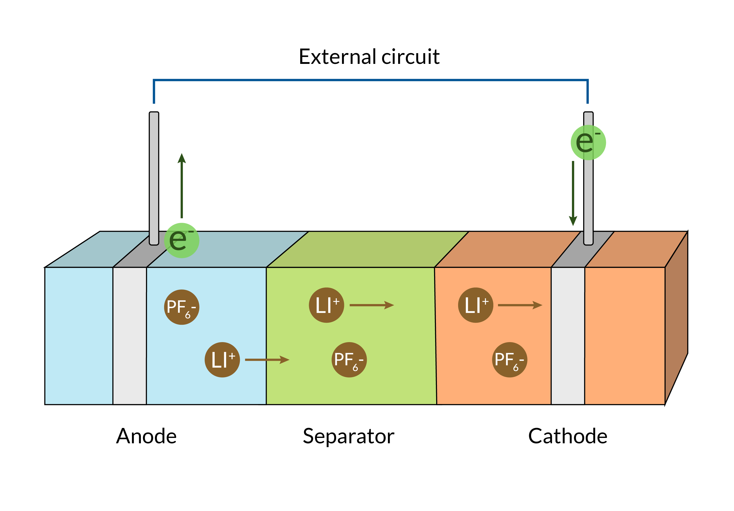 Figure 2. The structure of a lithium-ion battery.
The Doyle–Fuller–Newman model (Ref. 2) is the most commonly used model in LIB simulations. The electrode domains are treated as homogeneous when it comes to Li-ion transport but contain an additional dimension representing the radius of the electrode particles within the electrode domain. Hence, when modeling a battery in 1D, incorporating a radial dimension increases the dimension by one, thereby arriving at the common term “pseudo-2D” (Figure 3). Li-ions in the electrolyte solution act as charge carriers and transfer freely in the electrolyte solution.
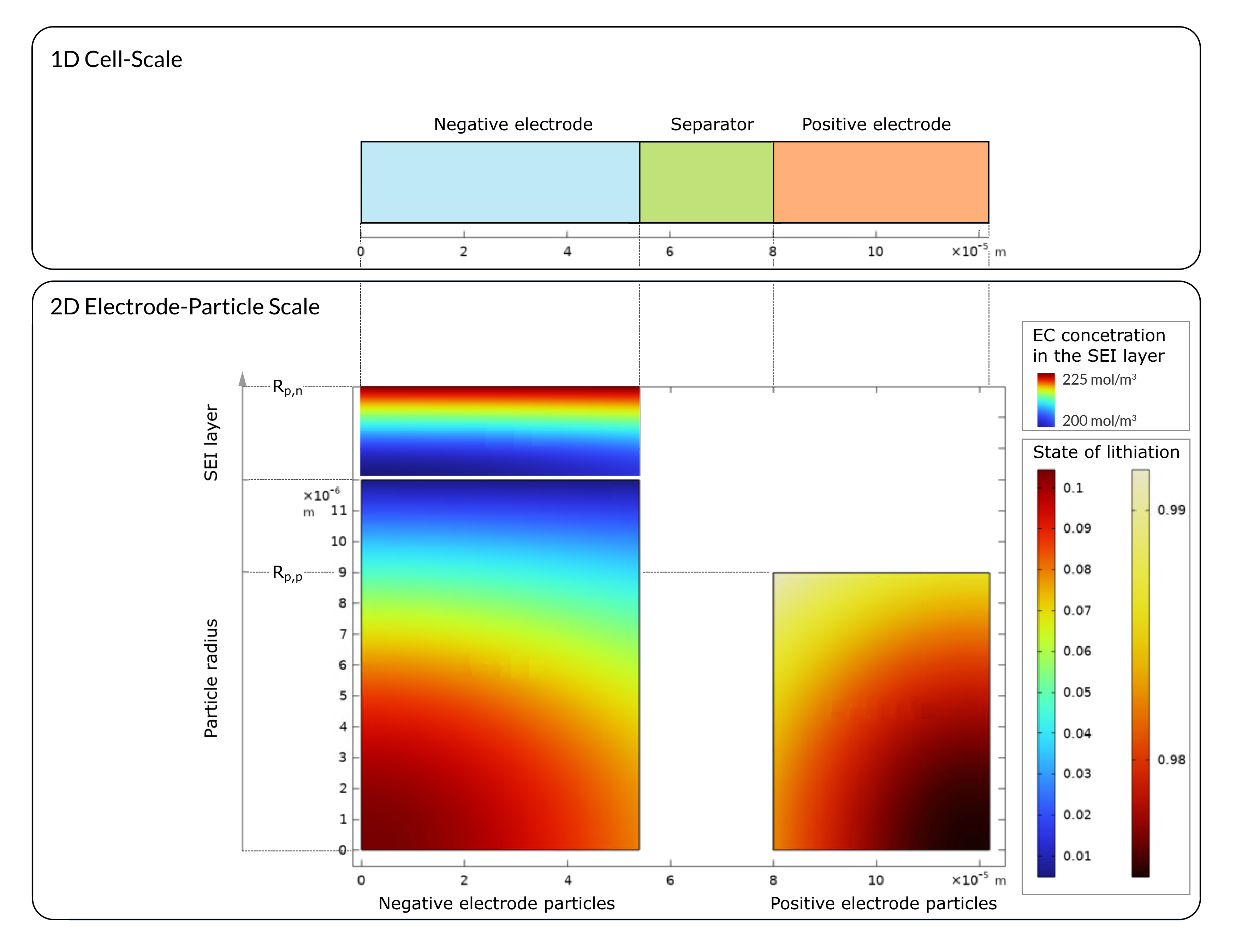
Figure 3. The pseudo two-dimensional (P2D) model of the lithium-ion battery, the DFN model. This multiscale model (cell and particle scales) is available in P2D, P3D, and P4D in the Battery Design Module. It is also available as a lumped P1D version.
When a battery discharges rapidly, lithium near the surface of the electrode particles is depleted faster than it can be replenished by diffusion from the interior. This imbalance causes a significant voltage drop and ultimately reduces the amount of energy available, especially at low temperatures since the diffusion rate will be rate limiting. Assuming spherical electrode particles, intercalated or deintercalated Li-ion reacts with the electrode particle surface at rate i_{tot,j}:
Intercalated lithium of concentration c_{P,j} diffuses inside the electrode particles of radius \delta_{P,j} (radial coordinate r) and diffusion coefficient D_{eff,S,j}. F is the universal Faraday’s constant, t is time, and j is an index representing the anode (j=n) or cathode (j=p) in order to differentiate between the physical properties of the domains.
Charge capacity will decrease over time for an LIB. Depending on its operating history, the internal resistance increases due to several degradation mechanisms. For the capacity and power loss observed over time, some of the important factors are the temperature, state of charge, and load profile. Because of this, as the battery is used, both capacity and power loss occurs. The primary degradation mechanism considered is the solid electrolyte interphase (SEI) that is forming during the charge–discharge cycles of a battery. By using the approach of Safari et al. from Ref. 3 the SEI formation can be modeled. Ethyl carbonate (EC) diffuses through the SEI layer and reacts at the electrode surface. SEI formation consumes electrolyte solvent and cyclable lithium (Figure 4). Other degradation mechanisms, such as lithium plating, cathode breakage, and electrode fracture, are not included in this work. To extend the 2D domain defined for the electrode particle, the SEI layer growth can be included using the following model:
This set of equations makes it possible to track the SEI layer thickness (degradation status), \delta_{SEI}, in any position of a battery using the growth rate \frac{d\delta_{SEI}}{dt}. The SEI layer thickness is assumed to be small compared to the particle radius, and the loss of lithium in the electrolyte is assumed to be small compared to the initial content. The spatially dependent solvent concentration in the SEI layer is c_{EC,P}, the diffusion coefficient D_{EC,P}, the electrolyte lithium concentration c_{solv}, and the SEI layer porosity \varepsilon_{SEI}. The consumption of Li-ion in the SEI layer formation contributes to i_{tot,j}.
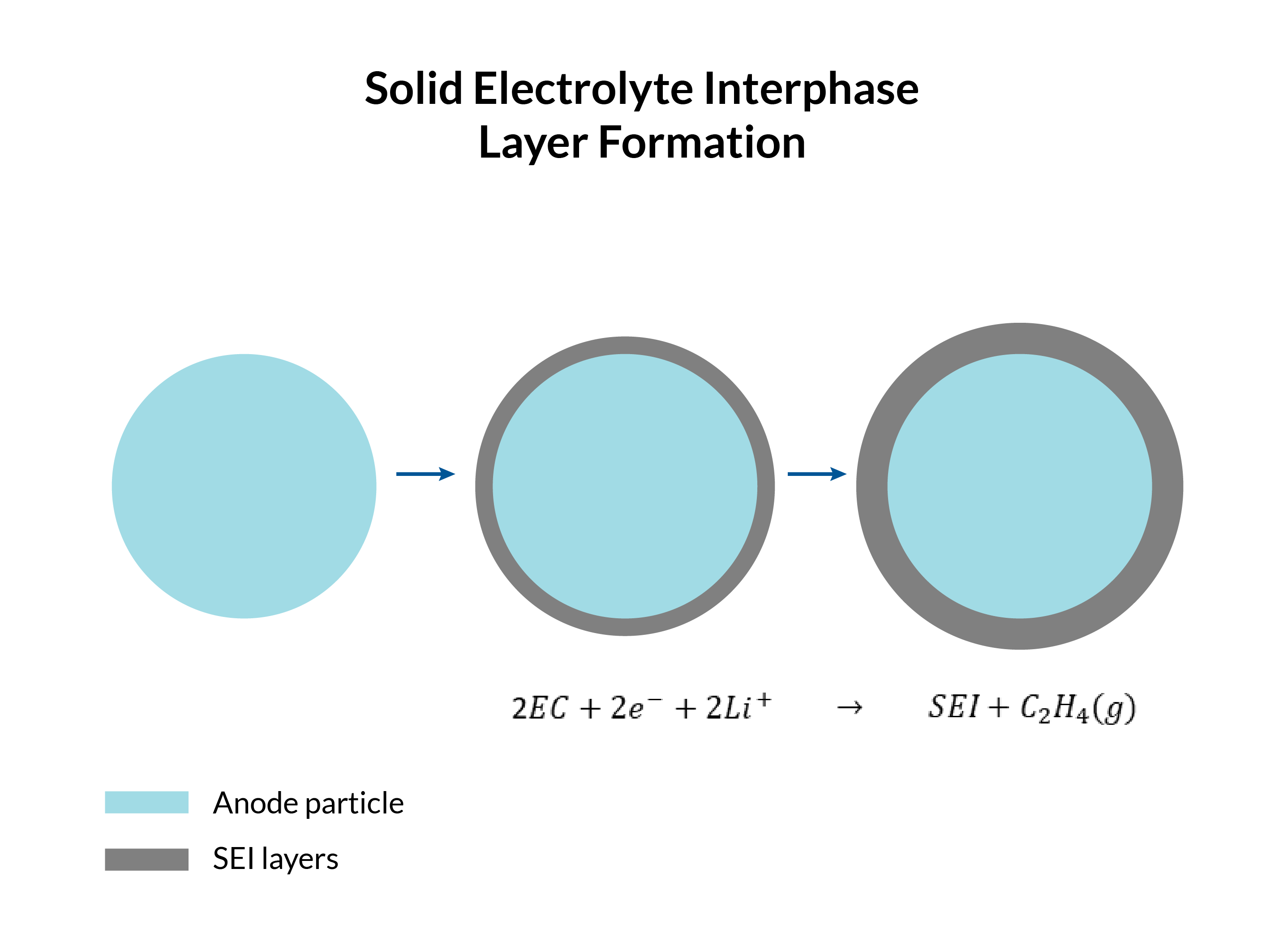
Figure 4. Battery degradation due to solid electrolyte interphase (SEI) formation.
Fitting Parameters to Real Data
Battery models involve a large number of physical parameters. Some of these parameters can be determined in controlled experiments, for example, by measuring heat transfer properties calorimetrically and electrode characteristics microscopically. Another subset of the parameters is considered as system-specific, and these parameters are fitted for experimental conditions of cycling performance of single-cell batteries. Databases like Battery Archive offer standardized and cleaned experimental data of various battery chemistries for various conditions, such as temperatures, charge current, discharge current, and state of health. System knowledge was used to devise a parameter-fitting strategy that allows sequential parameter fitting based on the data type. For example, the time series data of the first cycle was used to fit kinetic data to potential time data, and cycling time series data was used to estimate degradation parameters. Arrhenius-type expressions (two parameters) were used for the electrode diffusion coefficient and the exchange current density in the Butler–Volmer kinetics to account for temperature dependence.
Since the parameter fitting involves highly nonlinear dynamics and time integration, a brute-force method was adopted, where many samples based on a design of experiments defined by random samples were simulated, and the objective function (cost function) was evaluated for each simulation. The mean squared error between the simulated and experimental cell potentials was used as an objective function. Latin hypercube sampling (LHS) was used to sample from uniformly distributed parameter ranges.
A custom program was developed with the Application Builder in COMSOL Multiphysics® that allowed for automatically looping through parameter sets and datasets and reporting the objective function. Table A highlights the six experimental datasets, each consisting of hundreds of thousands of points in the time series. An excellent match was achieved for all datasets using the same parameter set. Figure 5 illustrates a comparison between the simulation and experimental degradation performance of a battery cell in terms of charge and discharge energy (W*h) and capacity (A*h).
| fID | Chemistry | Temperature | Charge Current | Discharge Current | SOC min. | SOC max. |
|---|---|---|---|---|---|---|
| 1 | NMC | Medium | High | High | Low | High |
| 2 | NMC | Medium | Low | Low | Low |
High |
| 3 | NMC | Low | Medium | Medium | Low |
High |
| 4 | NMC | Low | Low | Low | Low |
High |
| 5 | NMC | High | Medium | Medium | Low |
High |
| 6 | NMC | High | Low | Low | Low |
High |
Table A. The datasets included for parameter fitting with qualitative conditions.
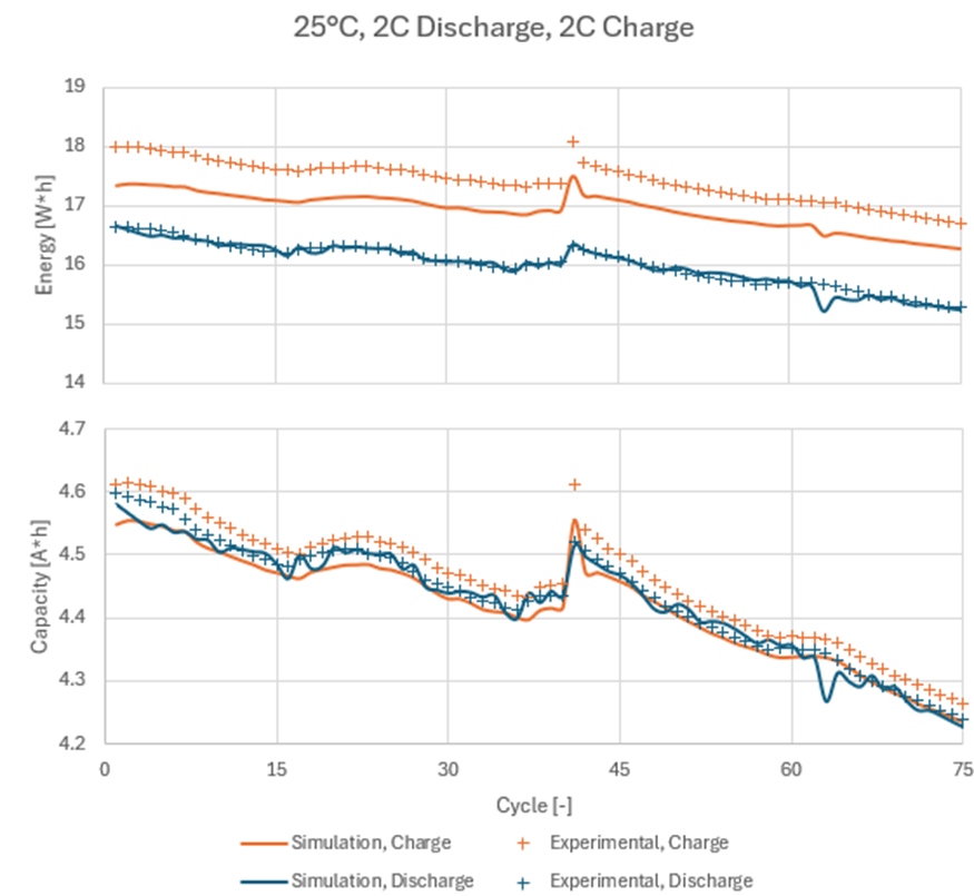 Figure 5. Cycling data for a single NMC battery cell, comparing simulated and experimental charge and discharge energy and charge and discharge capacity. Data source: Ref. 4.
Battery Simulation in 3D: Building Upon the Electrochemical Model
Many phenomena are only present in 3D, and to fully and accurately model these phenomena, the modeling therefore also needs to be expanded to 3D. This includes the modeling of, for example, the cooling on the side of the battery packs, the heating of the busbar, and the current distribution across many of the different individual batteries. Another aspect to consider is that temperature gradients across the battery pack can lead to spatially nonuniform degradation within the battery. An important thing to also note is that there are significant computational costs from going up in dimensions. Also, for the models at the scale of a full battery, it would not be possible to have the same level of detail as in the 1D chemistry, as the computational cost would simply be too great. Some of the information that was calculated in the 1D chemistry needs to be taken up in the full 3D model in order for it to accurately represent the functions of the battery, but much of the information is not needed at all. Therefore, the chemistry can likely be described with a reduced-order model, such that it is computationally feasible to include in a 3D model.
The DNN architecture that was implemented in COMSOL Multiphysics® version 6.1 was adopted in this work. For the most important inputs and outputs from the P2D model, in the span that we expect the model to run in, we are able to generate a dataset that was needed in the training of the DNN.
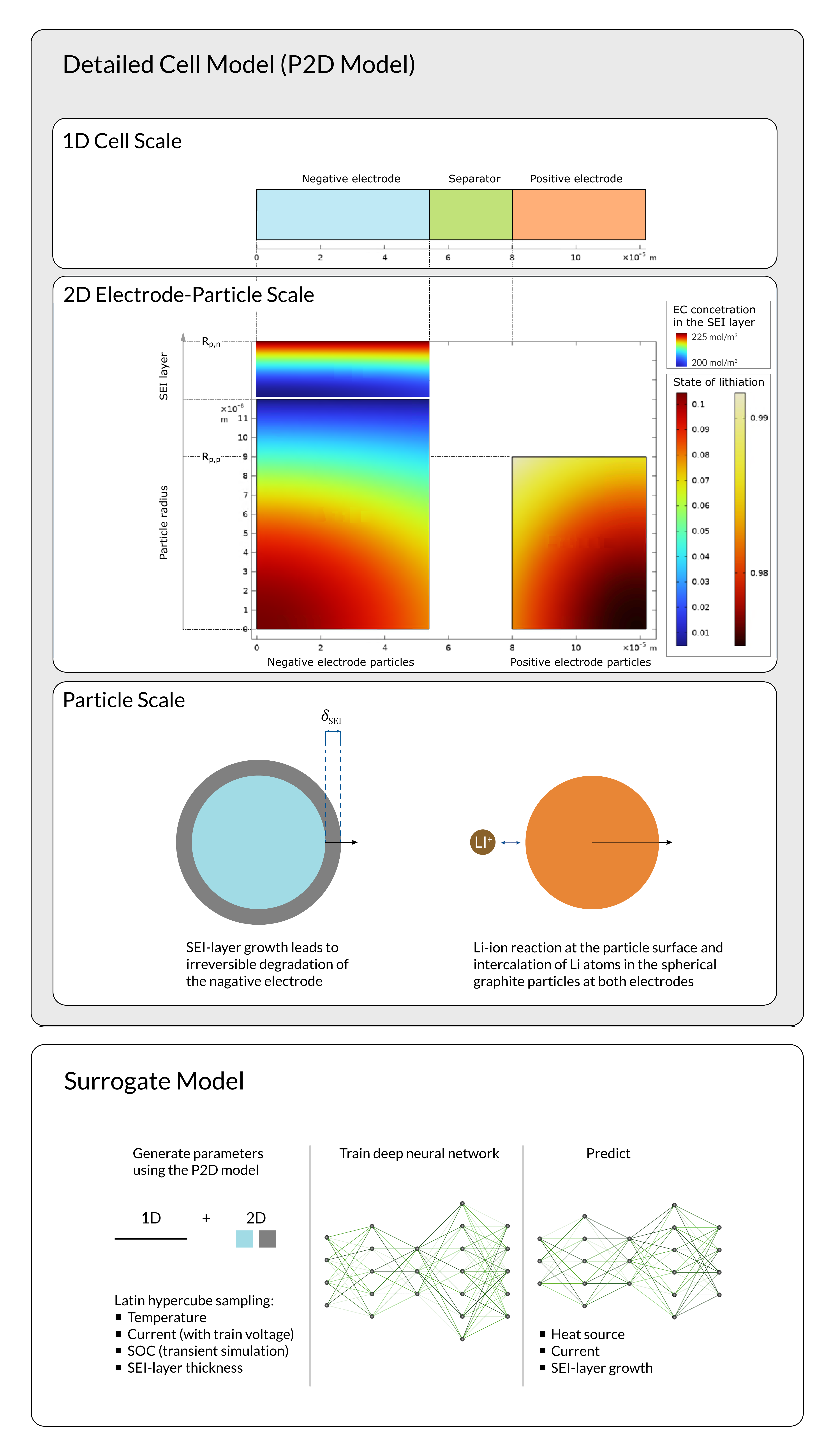
Figure 6. Conceptual workflow for data generation, DNN training, and approximation of the P2D model using a DNN-based surrogate model.
In order to obtain a representative span of the parameters (Figure 6), LHS was performed for the most important control parameters, the temperature, current (to be used with the recorded voltage to train the DNN), state of charge, and SEI layer thickness. While it is possible to make LHS in the Model Builder in COMSOL Multiphysics®, we opted to use the Method Editor in the Application Builder in order to control each individual simulation. That way, it was possible to distribute the simulation across many parallel COMSOL® sessions and collect the results automatically in one file. Moreover, this method allowed for reducing the time it would take to generate the necessary data each time some changes were made inside the P2D model. The scripting in the Application Builder also makes it easier to automate the entire sequence of operations, which would be beneficial if this was going to be packaged into an easy-to-use COMSOL model or potentially a COMSOL app to be used by clients.
After each iteration of solving for the P2D model, certain outputs were stored. Specifically, we chose values that would be integrated into the full 3D model, e.g., predicting the SEI layer growth speed in order to time integrate it into the SEI layer thickness.
Having this dataset, it was then a task of finding a configuration of the neural network in terms of activation functions, depth and width of the neuron layers that would give the most optimal performance, and learning rate. The DNN was evaluated against how closely it would predict the out-of-sample dataset. Another key performance metric was the time required to evaluate neural networks of a given width and depth. For example, having a very wide and deep DNN not only took a long time to train but also led to a significantly longer wait time for results.
Figure 7. Animation of a battery cell under fast discharge. From left to right: temperature, state of charge, and SEI layer thickness. The system exhibits spatial inhomogeneities due to a constant room-temperature boundary condition at the far-right end of the battery.
Figure 7 illustrates a 3D model and simulation that couple temperature, state of charge, and SEI layer thickness. The figure gives an indication of how much stress the battery is undergoing during its use. Among other things, the results also illustrate how the heat is developed and distributed inside the battery and how different areas inside the battery degrade in terms of SEI layer growth. This is a coupled dynamic effect: degradation alters future charge–discharge behavior, which modifies the temperature field and, in turn, drives further degradation through SEI growth.
For the system in Figure 7, temperature gradients lead to spatial variations in both the discharge rate and SEI layer growth.
Larger Battery Packs and Multiphysics Modeling
In practical applications, batteries are typically operated as part of packs rather than individually (Figure 8). It therefore becomes much more interesting to model entire packs of batteries. Specifically, the modeling could be performed for battery packs for an electric vehicle (EV). Modeling the full battery module or pack increases computational cost but provides a more accurate representation of thermal behavior and degradation during operation. By including flow and current distributions in the model, it gives a more realistic picture of how heat is generated and cooled in the system. By computing the temperature and state of charge, the model can predict where SEI deposition and associated degradation occur within the battery. Nonuniform temperatures across the battery pack lead to nonuniform degradation.
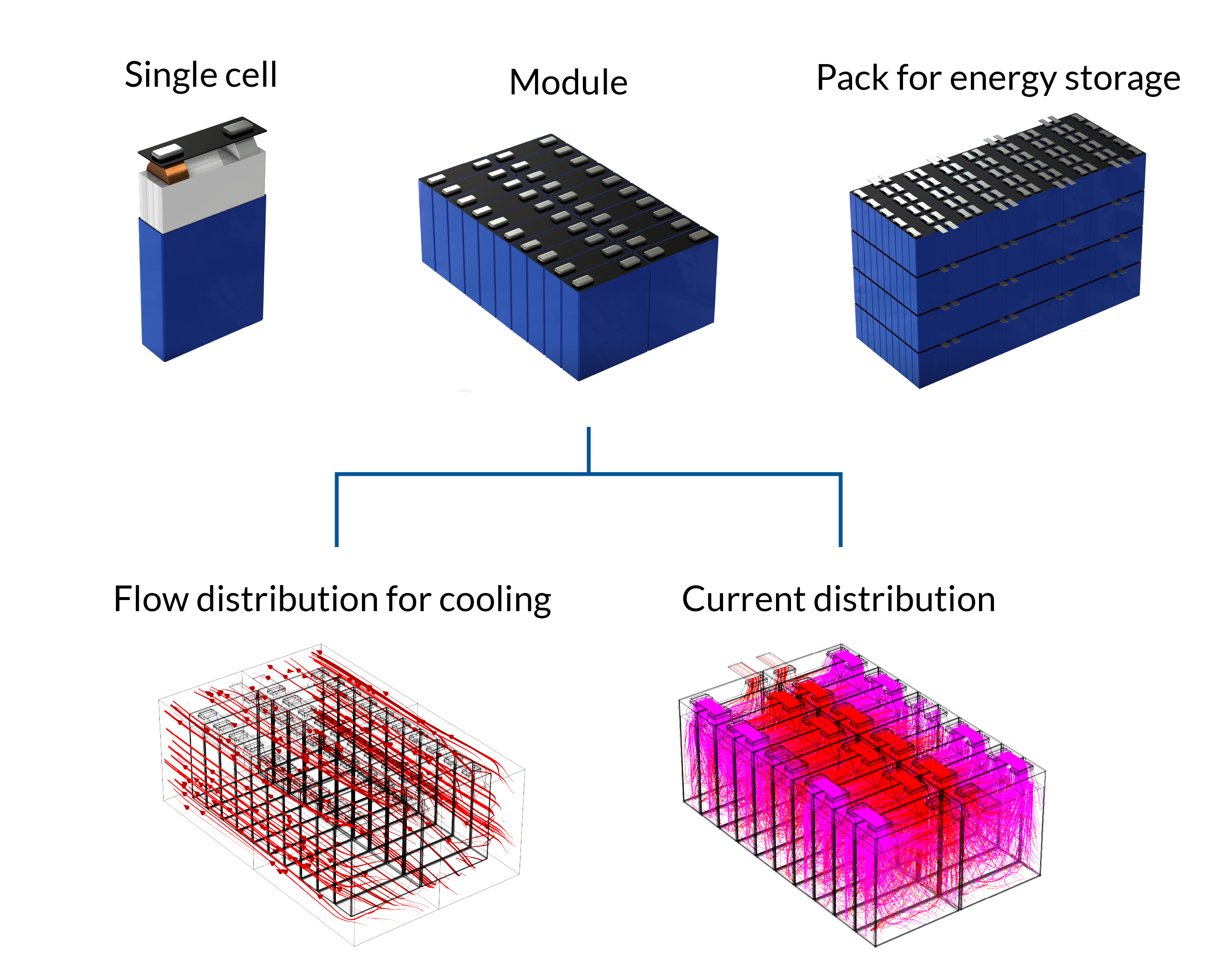 Figure 8. The figure illustrates the scaling of a battery system from a single cell to a module and a full battery pack for energy storage. It also highlights the phenomena that can be more accurately captured at the module and pack levels, including flow, current distribution, and ohmic losses and heating.
The current, temperature, state of charge, and SEI layer thickness are all modeled using the Weak Form PDE interface in COMSOL Multiphysics®.
Flow and temperature around the pack are modeled using the fluid flow and heat transfer interfaces in the CFD Module and Heat Transfer Module. The flow and temperature fields are coupled in the domain, while fixed-temperature and no-slip boundary conditions are imposed.
Figure 9. Animation of a battery module under fast discharge. From left to right: temperature, state of charge, and SEI layer thickness. A constant room-temperature boundary condition at the outer edges of the module leads to spatial inhomogeneities.
From these models (Figure 9), we can see that we can calculate temperature, charge, and SEI layer degradation distributions in the batteries. This information can provide battery pack manufacturers with valuable insight into how to run their systems as well as the lifetime expectancy.
Summary
By using surrogate models in COMSOL Multiphysics®, we are able to simulate large systems while retaining key electrochemical behavior that would otherwise be computationally infeasible. This has enabled us to obtain information on full battery packs and how they evolve over multiple charges and discharges, as well as how degradation evolves throughout the system. This information can be used to gain important learnings before the battery is put into production or undergoes a several-thousand-hour test.
The modeling technique we presented here is not unique to batteries. The methodology can be applied to a wide range of systems that differ in their underlying physics but share similar computational challenges, such as large scales and long transient behavior. In such cases, the surrogate modeling and DNN functionality in COMSOL® can indeed be an important tool for investigations.
About the Authors
André Gugele Steckel is a senior modeling specialist at resolvent, a COMSOL Certified Consultant based in Denmark. He holds an MSc in physics and nanotechnology and a PhD in engineering physics from the Department of Physics at the Technical University of Denmark (DTU). His work spans multiphysics simulation, with a particular emphasis on acoustofluidics, electromechanical and piezoelectric transducers, and thin-film technologies. He has contributed to COMSOL Conference proceedings on battery modeling, covering topics such as methods for predicting lifetime degradation and analyzing the impact of operation and manufacturing processes on battery performance using high-fidelity models and surrogate models.
Thomas Bisgaard was a senior simulation specialist at resolvent. He holds an MSc and a PhD in chemical engineering from DTU. His expertise spans multiphysics and multiscale mathematical modeling, process dynamics, optimization, and control, with doctoral research focused on heat-integrated distillation and optimal control. He has contributed to technical work on battery performance and lifetime modeling, combining mechanistic electrochemical models with surrogate approaches to assess the impact of operation and manufacturing processes.
References
- “Trends in batteries,” IEA; https://www.iea.org/reports/global-ev-outlook-2023/trends-in-batteries
- M. Doyle, T.F. Fuller, and J. Newman, “Modelling the Galvanostatic Charge and Discharge of the Lithium/Polymer/Insertion Cell,” Journal of the Electrochemical Society, 140(6), 1993; https://iopscience.iop.org/article/10.1149/1.2221597/pdf
- M. Safari et al., “Multimodal Physics-Based Aging Model for Life Prediction of Li-Ion Batteries,” Journal of the Electrochemical Society, 156(3): 2009, A145-153; https://iopscience.iop.org/article/10.1149/1.3043429
- Battery Archive; http://www.batteryarchive.org/
Additional Resources from Resolvent
To learn more about the topic discussed in this blog post, as well as the work of Resolvent, see:
- “Extending battery pack lifetime using virtual design and testing”, an article by Resolvent
- Resolvent’s COMSOL Certified Consultants page
Acknowledgements
The authors would like to acknowledge the financial support by the European M-ERA.NET 3 call (project9468 LaserBATMAN), Innovation Fund Denmark (grant number 1139-00001), and the Swedish Governmental Agency for Innovation Systems (Vinnova grant number 2022-01257). The project aims to optimize battery pack manufacturing with a focus on joining processes. The consortium is comprised of the following companies and institutions: University of Skövde (Sweden), Technical University of Denmark (Denmark), Volvo Group Trucks Operations (Sweden), Aurobay Powertrain Engineering Sweden (Sweden), and Resolvent (Denmark).


Comments (0)