
In this blog post we introduce the two classes of algorithms that are used in COMSOL to solve systems of linear equations that arise when solving any finite element problem. This information is relevant both for understanding the inner workings of the solver and for understanding how memory requirements grow with problem size.
Linear Static Finite Element Problem
Let’s consider a linear static finite element problem composed of three nodes and three elements:
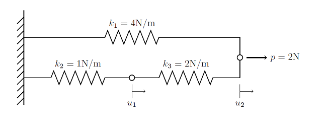
Each element is bounded by two nodes. One of the nodes is at the rigid wall, where we know the displacement will be zero, so we do not need to solve for that node. As we saw in the earlier blog post on linear static finite element problems, we can write a balance of forces for each node:
and we can write this as:
or even more compactly as:
We can solve this problem using the Newton-Raphson iteration method, and since this is a linear static problem, we can solve it in one iteration and using an initial value of \mathbf{u}_{init}=\mathbf{0}, giving us this solution:
Now, this problem only has two unknowns, or degrees of freedom (DOF), and can easily be solved with pen and paper. But in general, your matrices will have thousands to millions of DOF’s, and finding the solution to the above equation is usually the most computationally demanding part of the problem. When solving such a system of linear equations on a computer, one should also be aware of the concept of a condition number, a measure of how sensitive the solution is to a change in the load. Although COMSOL never directly computes the condition number (it is as expensive to do so as solving the problem) we do speak of the condition number in relative terms. This number comes into play with the numerical methods used to solve systems of linear equations.
There are two fundamental classes of algorithms that are used to solve for \bf{K^{-1}b}: direct and iterative methods. We will introduce both of these methods and look at their general properties and relative performance, below.
Direct Methods
The direct solvers used by COMSOL are the MUMPS, PARDISO, and SPOOLES solvers. All of the solvers are based on LU decomposition.
These solvers will all arrive at the same answer for all well-conditioned finite element problems, which is their biggest advantage, and can even solve some quite ill-conditioned problems. From the point of view of the solution, it is irrelevant which one of the direct solvers you choose, as they will return the same solution. The direct solvers differ primarily in their relative speed. The MUMPS, PARDISO, and SPOOLES solvers can each take advantage of all of the processor cores on a single machine, but PARDISO tends to be the fastest and SPOOLES the slowest. SPOOLES also tends to use the least memory of all of the direct solvers. All of the direct solvers do require a lot of RAM, but MUMPS and PARDISO can store the solution out-of-core, which means that they can offload some of the problem onto the hard disk. The MUMPS solver also supports cluster computing, allowing you to use more memory than is typically available on any single machine.
If you are solving a problem that does not have a solution (such as a structural problem with loads, but without constraints) then the direct solvers will still attempt to solve the problem, but will return an error message that looks similar to:
Failed to find a solution.
The relative residual (0.06) is greater than the relative tolerance.
Returned solution is not converged.
If you get this type of error message, then you should check to make sure that your problem is correctly constrained.
Iterative Methods
The iterative solvers in COMSOL encompass a variety of approaches, but they are all conceptually quite simple to understand at their highest level, being essentially similar to a conjugate gradient method. Other variations include the generalized minimum residual method and the biconjugate gradient stabilized method, and there are many variations on these, but they all behave similarly.
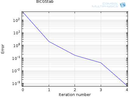
Contrary to direct solvers, iterative methods approach the solution gradually, rather than in one large computational step. Therefore, when solving a problem with an iterative method, you can observe the error estimate in the solution decrease with the number of iterations. For well-conditioned problems, this convergence should be quite monotonic. If you are working on problems that are not as well-conditioned, then the convergence will be slower. Oscillatory behavior of an iterative solver is often an indication that the problem is not properly set up, such as when the problem is not sufficiently constrained. A typical convergence graph for an iterative solver is shown below:
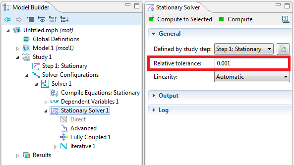
By default, the model is considered converged when the estimated error in the iterative solver is below 10-3. This is controlled in the Solver Settings window:
This tolerance can be made looser, for faster solutions, or tighter, for greater accuracy on the current mesh. The tolerance must always be greater than a number that depends on the machine precision (2.22×10⁻¹⁶) and the condition number (which is problem dependent). However there is usually no point in making the tolerance too tight since the inputs to your model, such as material properties, are often not accurate to more than a couple of digits. If you are going to change the relative tolerance, we generally recommend making the tolerance tighter in increments of one order of magnitude and comparing solutions. Keep in mind that you are only solving to a tighter tolerance on the mesh that you are currently using, and it is often more reasonable to refine the mesh.
The big advantage of the iterative solvers is their memory usage, which is significantly less than a direct solver for the same sized problems. The big disadvantage of the iterative solvers is that they do not always “just work”. Different physics do require different iterative solver settings, depending on the nature of the governing equation being solved.
Luckily, COMSOL already has built-in default solver settings for all predefined physics interfaces. COMSOL will automatically detect the physics being solved as well as the problem size, and choose the solver — direct or iterative — for that case. The default iterative solvers are chosen for the highest degree of robustness and lowest memory usage, and do not require any interactions from the user to set them up.
Concluding Thoughts on Direct and Iterative Solution Methods
When solving the systems of linear equations of a simulation, COMSOL will automatically detect the best solver without requiring any user interaction. The direct solvers will use more memory than the iterative solvers, but can be more robust. Iterative solvers approach the solution gradually, and it is possible to change the convergence tolerance, if desired.


Comments (7)
Anu Das
October 7, 2015i tried to couple poisson eqn and transport of diluted species. but it didn’t converge. below is the brief notes on how i attempt to solve it :
( 3D geometry is needle-plate electrode ) but i used 2D axis symmetric [took only the boundary of needle tip which is at 1 KV , rise time 1e-6 us and lower plate being at 0 V using electrostatics.
charge continuity eqn i.e del(rhe)/del(t) + div(-rhe *meu*E) = A*E*exp(-B/E) using transport of diluted species.
BC used is convective flux is zero at electrode boundary. i.e n.grad(rhe) = 0
coupling the two physics via space charge density > rhe in electrostatics
used PARDISO, time range [0,1e-8,1e-7]. Model didn’t converge. Plz send me your tips to tackle this problem.
Walter Frei
October 14, 2015 COMSOL EmployeeHello Anu,
Those questions fall rather outside of the scope here. Instead, you would want to contact your COMSOL Support Team directly for assistance.
Moez El-Massry
March 2, 2016Could I manually make the solver use direct or Iterative solution methods? (as I am doing a simulation that stops and report an error “out of memory during LU factorization”, and according to the blog the direct solution method may help.)
Nicholas Goldring
June 8, 2016I actually have the exact same question. I would like to manually select a solver that takes less memory as I am currently getting the same error message.
Walter Frei
June 9, 2016 COMSOL EmployeeHello,
With respect to out-of-memory questions, please see this KB:
https://www.comsol.com/support/knowledgebase/1030/
Bastián Rodríguez López
May 12, 2020Hi! Thank you for the explanation. I am trying to simulate an aluminum two pieces hardware with contact points between them. I would like to know which one of the solvers I should use. Which one is an explicit way and one is an implicit? Thank you in advance.
Jinsub Park
April 24, 2024Nice explanation