
If there is one number to rule all of math and science, it is arguably pi. This little symbol, π, has a big history, dating back thousands of years. From ancient civilizations making crude approximations over circles to modern-day supercomputers calculating trillions of digits, pi has captured the imaginations of mathematicians and curious minds alike. In this blog post, let’s turn to a fun and popular approach to calculating pi using the features available in the COMSOL Multiphysics® simulation software.
Approximations of Pi Through Time
The earliest known approximations of pi are found in ancient civilizations. Mathematicians from Babylon had approximated pi to 3, which was reasonable to carry out architectural projects at the time, before refining it to a value of 3.1251. Mathematicians in Egypt and scholars in India provided similar values by comparing the area of a circle and an octagon2 and astronomical calculations3, respectively. A significant breakthrough was made by Greek scholars, including Archimedes, who used geometric methods to approximate pi to within 3 orders of magnitude of accuracy4.


Left: Archimedes Thoughtful, 1620 (also known as Portrait of a Scholar) by Domenico Fetti. Image in the public domain, via Wikimedia Commons. Right: A portrait of Leonardo Fibonacci. Image in the public domain, via Wikimedia Commons.
The popular approximation of 3.14 that we all use today comes from the Chinese mathematician Liu Hui, who suggested it for practical purposes5. Subsequent developments in pi’s calculation involved evaluating infinite series and exploiting trigonometric relations. Using calculus, mathematicians were able to derive infinite series that could be used to calculate pi to a high degree of accuracy with key contributions made by Fibonacci and Al-Khwarizmi.
These developments laid the foundation for modern methods in use today, including those used in computer algorithms to calculate pi with an extremely high precision through advanced mathematics and computing power to compute trillions of digits. Some notable computational methods include the Chudnovsky algorithm, the Gauss–Legendre algorithm, Machin’s formula, and notably: the Monte Carlo method.
The Monte Carlo Method, in Layperson’s Terms
The Monte Carlo method is a computational technique that relies on random sampling to estimate numerical results. It is particularly useful for problems with a large number of variables where an inherent randomness can be used to solve a deterministic problem. Imagine you’re trying to calculate how much pizza to order for a party. The deterministic problem here is to figure out how many slices each person will eat. Instead of asking each person how many slices they would have and summing the result (which can be quite cumbersome for a large party), what you could do is randomly pick a few friends, ask them how many slices they’d have, and then average it out to solve the problem. That’s a bit like the Monte Carlo method — using random samples to estimate a value. Monte Carlo methods are popularly applied to simulations of complex phenomena such as fluids, statistical mechanics, biochemistry, cryptography, sociology, and psychology.

The ideology can be extended to what is now a popular and fun way to estimate pi. This involves randomly placing points inside a square and counting how many lie within a circle inscribed in the square. The ratio of points inside the circle to the number of points in total can be used to approximate pi. Since the area of a circle inscribed in a square of side 2r is πr2 and the area of a square is (2r)2 = 4r2, the ratio of their areas is π/4. This means that the probability of a point landing inside the circle is π/4. Therefore, if we multiply the ratio of points inside the circle to the total points by 4, we get an estimate of π. The more points we use, the more accurate our estimate will be. This is because as the number of points increases, the ratio converges to the actual value of π/4.
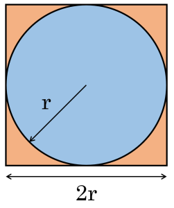
The foundation for estimating pi.
Estimating Pi Using the Monte Carlo Method in COMSOL Multiphysics®
To perform this simple Monte Carlo simulation, we will take advantage of the Mathematical Particle Tracing interface, which is available when you add the Particle Tracing Module to the COMSOL Multiphysics® software platform. Though users of this module typically do not use it to simply generate points randomly, we decided to use it for our fun example here for visualization and aesthetics purposes.
Now, onto the example. Particles are released randomly onto a square domain and remain stationary. The number of particles that lie within the inscribed circular region are tracked to provide a real-time estimate of pi. We see that the estimated value (solid blue line) approaches the true value (dashed green line) for an increasing number of points. It is important to note that the accuracy of the estimated value does not linearly vary with the number of points. The statistical error in the Monte Carlo approximation typically is proportional to 1/sqrt(n). This means that to decrease the error by a factor of 10, you typically need to increase the number of points by a factor of 100.
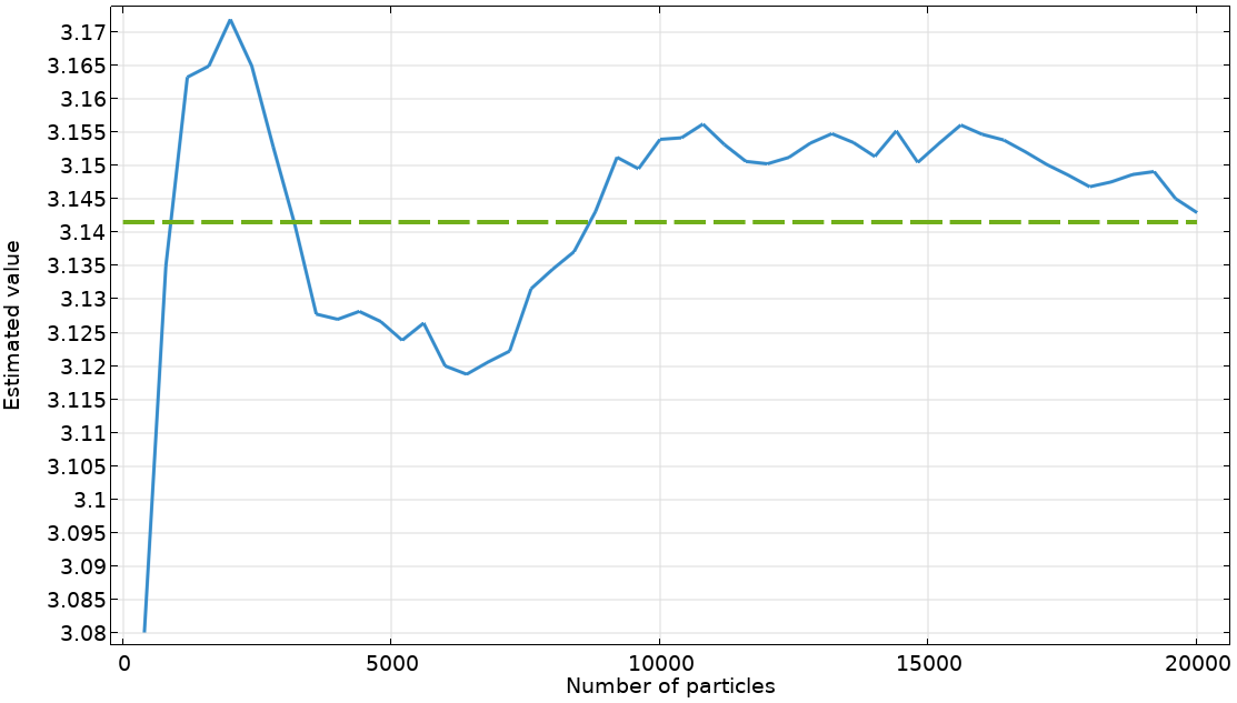
A comparison of the real-time estimate of pi (solid blue line) and its true value (dashed green line) for an increasing number of randomly placed points.
Next, we used the Application Builder in COMSOL Multiphysics® to create an app based on the model. The app makes it possible to vary the number of points using a slider and we get the real-time estimated value of pi and the error from the true value. The app also visualizes the randomly placed points, which are color coordinated to identify the ones that lie within the circle.
A screen recording of someone using the app to estimate pi based on different numbers of points and get a visual interpretation of the results.
Next Steps
You are welcome to download the MPH file with the app design and related files from the Application Gallery here: Using the Monte Carlo Method to Estimate the Value of Pi.
- More models that use the Monte Carlo method:
- An example that demonstrates how to perform a direct Monte Carlo simulation of the Ishigami function
- A model that uses the Monte Carlo method to evaluate the performance of a simple turbomolecular pump in the free molecular flow regime
- A model that computes the transmission probability through an s-bend geometry using the Monte Carlo method
- Information about the Application Builder:
- See what our customers have to say about the Application Builder in the blog post titled “Multiphysics Simulation Is More Accessible with the Application Builder“
- Read about a smartphone app powered by multiphysics simulation in the story titled “Forecasting Fruit Freshness with Simulation Apps“
- Take a look at how a university professor uses apps within the classroom in the story titled “Bringing Lab Courses to Remote Learning Students with Simulation Applications“
References
- P. Beckmann, A History of π. New York: St. Martin’s Press, 1971
- C. Rossi, Architecture and Mathematics in Ancient Egypt. Cambridge University Press, 2004
- C. Krishna, A profile of Indian culture. Indian Book Company, 1975
- D.B. Damini & A. Dhar, How Archimedes showed that pi is approximately equal to 22/7. arXiv e-prints, 2020
- Y. Lam & T.S. Ang, Circle measurements in ancient China, Historia Mathematica, 1986


Comments (0)