
In many features in the COMSOL Multiphysics® software, you have the option to use a weak constraint. In this blog post, we will take a deeper look at what a weak constraint is, why you may want to use it, and what special considerations you may need to make when using it.
Table of Contents
- How Do You Implement Weak Constraints in COMSOL Multiphysics®?
- Lagrange Multipliers
- Finite Element Constraint Handling
- Introducing the Lagrange Multipliers
- Weak Constraints
- Nitsche Constraints
- A Note on Terminology
- Interpretation of Lagrange Multipliers
- Things to be Aware of When Using Weak Constraints
How Do You Implement Weak Constraints in COMSOL Multiphysics®?
The default type of constraint in COMSOL Multiphysics® is, in almost all cases, a pointwise constraint. A pointwise constraint is applied directly to a degree of freedom (DOF), typically on a set of nodes in the mesh.
In the settings for most standard constraints features in the Model Builder, there is a section called Constraint Settings. This section is where you can choose between different constraint formulations. For some features, the list may contain a third option, a Nitsche constraint.
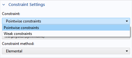
Example of a Constraint Settings section.
However, this section is not displayed by default. Weak constraints are among the features that are considered “advanced”. You can enable this section by selecting Advanced Physics Options in the Show More Options dialog.
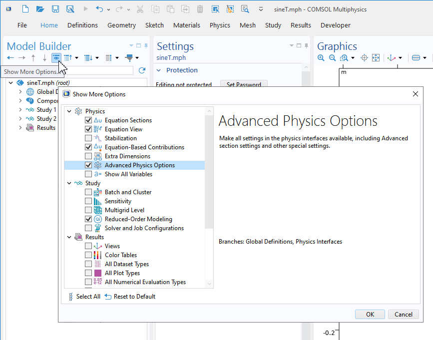 Enabling Advanced Physics Options.
Lagrange Multipliers
Since weak constraints are based on Lagrange multipliers, it seems prudent to start with some general information about that topic.
The concept of Lagrange multipliers was introduced by mathematician Joseph-Louis Lagrange as part of his work on variational calculus. Learn more about his life and work in our blog post “Happy Birthday, Joseph-Louis Lagrange”.
A general constrained minimization problem can be formulated as follows: Find the minimum of a function f(\mathbf x) \;\text{for} \; \mathbf x \in \Omega, subject to a set of constraints g_i(\mathbf x) = 0. The problem is then how to, in a general way, fulfill the constraints. For trivial constraints (for example, linear constraints), it may be possible to explicitly invert the constraint expressions and insert the result into f(\mathbf x), thus reducing the number of unknowns. But this is the exception rather than the rule.
The idea is now that you can instead find the minimum of
Here, \lambda_i is a set of new unknown variables, the Lagrange multipliers. Since g_i(\mathbf x) = 0 for the true solution, it is evident that the minimum value of \mathcal{L} equals the constrained minimum of f. But why does it work?
To find the extrema of a function, you need to compute the partial derivatives with respect to all variables and set them to zero. In this case,
and
Thus, the constraint equations are recovered by differentiating with respect to the Lagrange multipliers, meaning the constraints remain active. The first set of equations, however, is more subtle. Understanding why they ensure a correct minimum for certain values of \lambda_i requires a more detailed argument. Notably, the new equations now also involve the gradients of the constraint functions.
For a full explanation, together with some elucidating examples, see: “Lagrange multiplier”.
Finite Element Constraint Handling
Let’s consider a simple linear static finite element problem. On the final discretized matrix form, it can be written as
where \mathbf{K} is the stiffness matrix, \mathbf {u} is the vector of degrees of freedom, and \mathbf {f} is the vector of nodal loads. In order to be able to solve this system (make the stiffness matrix nonsingular), a minimum number of degrees of freedom must have known values. For a heat transfer problem, at least one temperature is required, while for a solid mechanics problem in 3D, at least 6 displacements degrees of freedom must be known. Most commonly, such values are given by a direct input of that DOF. There are also other options, such as a convection boundary condition in heat transfer analysis or spring conditions for structural mechanics.
Often, many more constraints than necessary for stability are applied, such as over a whole boundary. As long as there are some constrained degrees of freedom, the system of equations can then formally be partitioned as
Here, the subscript “a” indicates an active DOF, and the subscript “c” indicates a constrained DOF. The vector \mathbf {r} contains the, yet unknown, reactions at the constrained nodes. This terminology comes from solid mechanics, where it is natural to talk about reaction forces. In, for example, heat transfer, the reaction is a heat flux. In most cases, no loads, \mathbf f_{\mathrm{c}}, are applied at constrained nodes, since they have no effect on the solution.
The values of \mathbf u_{\mathrm{c}} are known, say \mathbf u_{\mathrm{c}}= \mathbf u_0. The most basic way of handling this when solving the finite element equations is to solve only for the active DOFs. The effects of the prescribed values can be moved to the right-hand side, leaving
Once the reduced system of equations has been solved, it is possible to compute the reactions during a results evaluation step using
In practice, it is only the matrix \mathbf k_{\mathrm{aa}} that needs to be assembled. The other forward multiplications can be handled more efficiently at the element level.
This way of expressing the reaction forces assumes a linear problem so that the matrices are constant. A more general formulation is to say that the reaction forces are a result of the computation of residuals. For active degrees of freedom, the residuals for a converged solution are small. At constrained nodes, the residuals are larger and can be interpreted as reaction forces.
Computing the nodewise reactions a posteriori is essentially what you can do using the reacf() operator in COMSOL Multiphysics®. Note that the values you get are concentrated nodal values. It is not a distributed field. Depending on the shape functions used in the element, such nodal values can have a quite nonintuitive distribution. The sum is exact down to the level of numerical roundoff.
A downside of this approach is that if you need to make use of the reactions inside the computations, they would not be available.
Note: The description above is based on finite element formulations in general and is a strong simplification of what really goes on inside COMSOL Multiphysics®. The constraint handling is far more complex. For example, constraints may be nonlinear or connect different variables, even those representing different physical fields.
Introducing the Lagrange Multipliers
For now, we will stay on the discretized form. To be less abstract, consider an example from solid mechanics. For a linear problem, it can be shown that the potential energy is
Minimizing W with respect to the displacements will retrieve the ordinary set of equations used earlier. Now, let’s augment the potential by adding all constraints multiplied by individual Lagrange multipliers:
For clarity, the DOF vector is split into unconstrained (\mathbf u_{\mathrm{a}}) and constrained (\mathbf u_{\mathrm{c}}) DOFs. It is important to note that in this new formulation, the constrained DOFs are considered as unknown. This is a fundamental difference from the previous approach.
For simplicity, it has been assumed that no loads act on the constrained DOFs. Differentiating with respect to each set of DOFs now gives the following system of equations:
Using the second row of equations, it can easily be verified that the Lagrange multipliers are identical to the nodal reaction vector \mathbf {r}, introduced above. The last row of equations simply states that \mathbf u_{\mathrm{c}} = \mathbf u_0.
If the original stiffness matrix is symmetric (as is often the case), this new system of equations is also symmetric. There are, however, some downsides with this formulation:
- Instead of solving for only the active degrees of freedom, this formulation requires solving for the active DOFs, the constrained DOFs, and the Lagrange multipliers.
- There are zeros on the diagonal. Not all methods for solving linear systems of equations can deal with that.
- It becomes important to scale the equations properly for numerical reasons. The original stiffness matrix entries can be very far from unity.
With these drawbacks, why would a formulation like this be beneficial? Here are some reasons:
- The values of the reactions are actually a part of the problem formulation. That is, it is not enough to consider them as a result quantity.
- Strongly nonlinear constraints tend to converge better when formulated using Lagrange multipliers.
- It is not possible to use time derivatives in pointwise constraints. If you need that, the use of Lagrange multipliers is the only option.
Weak Constraints
Weak constraints are based on the same Lagrange multiplier concept. However, the constraints are considered already in the mathematical description before discretization.
The finite element formulation is based on using the weak form of the underlying equations. For solid mechanics, this is also known as the principle of virtual work. The formulation is as follows:
Here, \sigma is the stress tensor, \varepsilon is the strain tensor, \mathbf {t} is the traction vector, and \mathbf {u} is the displacement field. The symbol \delta indicates a variation operator. In COMSOL Multiphysics®, it is represented by the test() and var() operators. The sign convention is the one used in the program.
For simplicity, it is assumed that the loads (tractions) act only on the boundary. In a more general setting, there may also be volume, edge, and point loads.
To make the formulation complete, there will be prescribed values of the displacements on some part of the boundaries,
When approximating the displacements with selected shape functions, this mathematical expression will be transformed into the discretized form of the finite element equations.
Using the idea of Lagrange multipliers, the constraints can now be incorporated into the weak expression by adding an extra term:
Here, \lambda(\mathbf x) is a Lagrange multiplier field, defined over the constrained boundary. Assuming that \mathbf u_0 is just a prescribed value (independent of the solution), the last term can be expanded into three terms so that
When the weak form expression is transformed into discretized equations using the finite element method, \lambda(\mathbf x) is approximated using shape functions over the element, just as the displacements are. In principle, the shape functions for the two fields could be selected independent of each other, but then stiffness matrix symmetry would be lost (and the matrix may even become singular). Thus, the same shape functions as for the displacements are normally used. After assembly, the system of equations will look like
The matrices \mathbf L and \mathbf L^T stem from the third and fourth terms in the weak expression above, which have a symmetry property as long as the same shape functions are used for displacements and Lagrange multipliers.
Supplemental note: The matrix \mathbf L is actually identical to the mass matrix contribution that you would get from a unit mass per area distribution on the same boundary. In the Solids Mechanics interface, such a mass distribution can be given using an Added Mass node.
For comparison, the system of equations obtained when applying the Lagrange multipliers to the discretized system is repeated from above:
As can be seen, the structure is similar, but the unit matrices have been replaced by \mathbf L, and the right-hand side now contains \tilde {\mathbf u}_0, which is a weighted form of \mathbf u_0.
So, what is the effect of this modification? Well, the nodal values of the prescribed DOFs will no longer be exactly what was prescribed. On the other hand, the values between the nodes will, in an average sense, be closer to the given function \mathbf u_{0}(\mathbf x).
To illustrate this, let’s consider a simple example from heat transfer that compares the results obtained using both the standard pointwise constraint method and the weak constraint method.
Example One: Heat Transfer
A 2D heat transfer problem is solved on the unit square with a 2×2 mesh using second-order Lagrange elements. On the rightmost boundary, the temperature is prescribed as sin(2*Y). On the opposite boundary, the temperature is set to zero. On the remaining boundaries, there are no boundary conditions, corresponding to no flux. The prescribed temperature is chosen so that it cannot be exactly described by the quadratic shape functions.
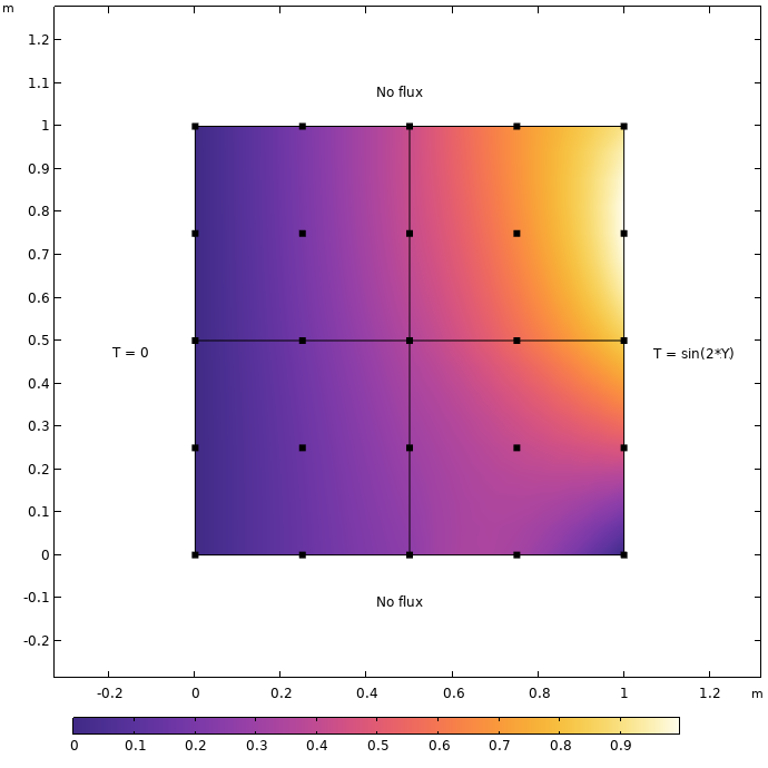 The model, with boundary conditions and a computed temperature field.
If we plot the temperature along the rightmost edge, the difference between the two methods is hardly visible, as can be seen in the image below.
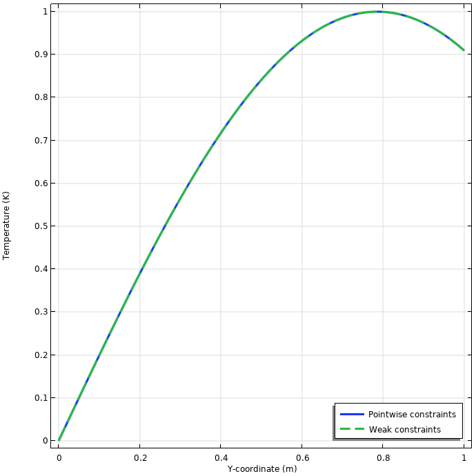 The temperature distribution along the rightmost edge.
In the figure below, we see a comparison between the temperature and its prescribed value, which offers a more interesting plot.
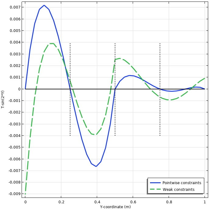 A plot of the difference between the actual temperature field and the prescribed temperature. The locations of the node points are indicated by dashed vertical lines.
Here, it can be seen that pointwise constraints exactly match the given function at the node points. This is not the case when using weak constraints.
Is one or the other solution better? A first attempt could be to compute the average error, when compared to the given function. The result is given in the table below.
| Constraint | Average of T-sin(2*Y) |
|---|---|
| Pointwise constraint | 2.5*10-4 |
| Weak constraint | 3.6*10-7 |
It turns out that the mean error is three orders of magnitude smaller when using the weak constraints. By adding the Lagrange multiplier field, the prescribed value will be matched as good as possible, in an average sense. To check that this is not a happy coincidence, a parametric sweep is performed where the mesh density along the edge is changed from 1 to 20 elements.
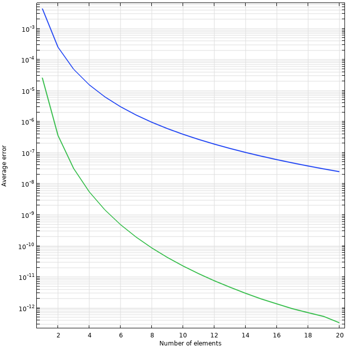 The average error in temperature along the rightmost edge as a function of mesh density.
It should not be forgotten that these errors are very small. For any reasonably fine mesh, these comparisons are interesting only from a theoretical point of view.
In the next example, the effects of a chosen constraint type will be directly visible.
Example Two: Bar Model
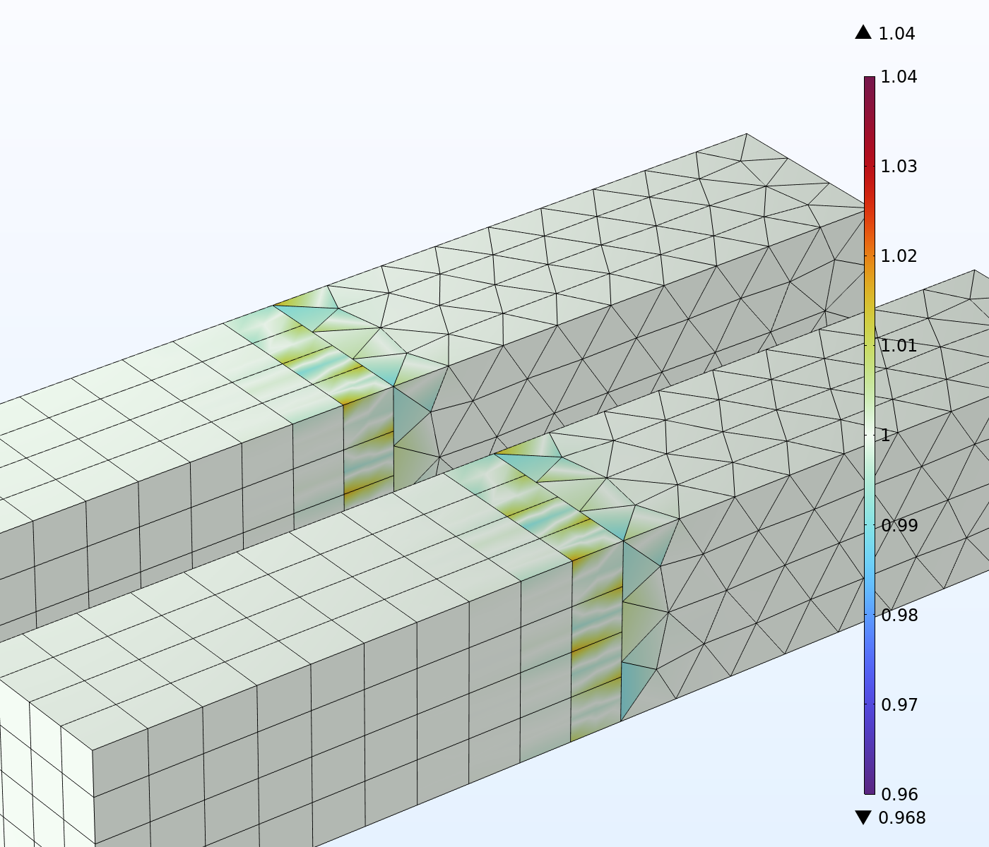
In this example, we are working with a bar that has a square cross section and is subjected to uniaxial tension. This is an assembly with two domains. One domain is meshed with hexahedral elements, and the other is meshed with tetrahedral elements. Since it is an assembly, the two domains are joined using a Continuity condition. The effect is that the mesh is nonconforming at the common boundary.
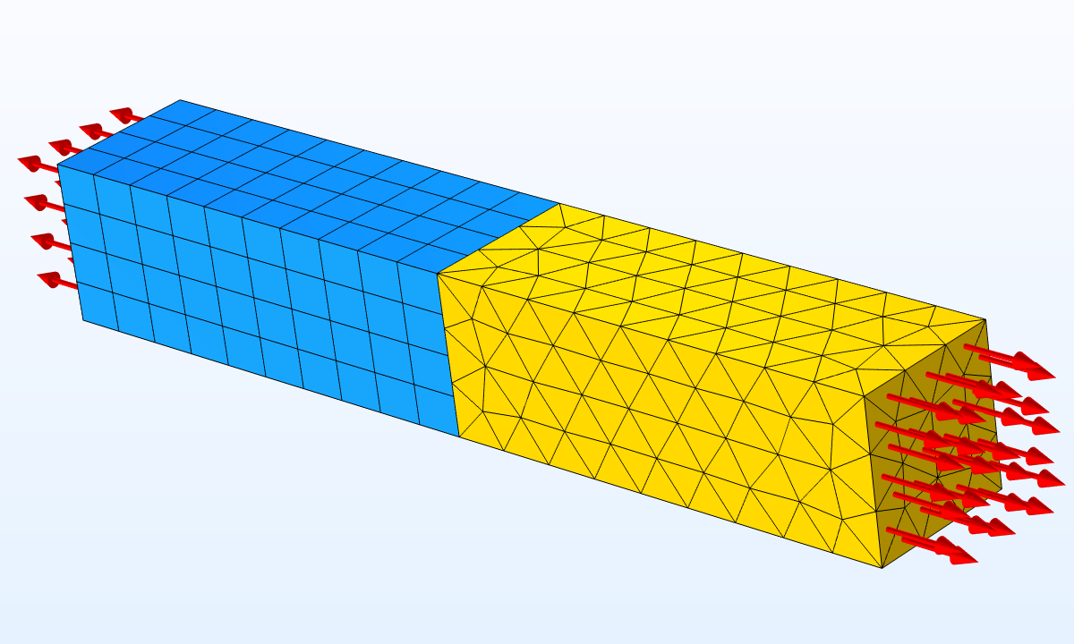 The mesh and loading of the bar model.
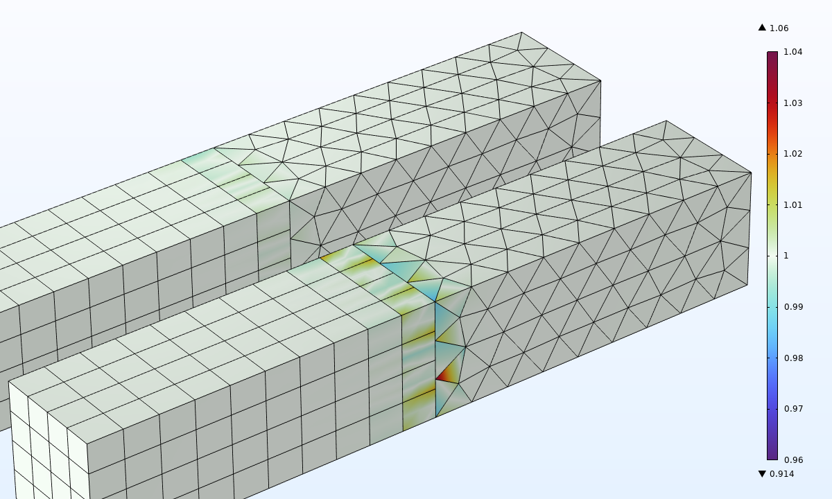
As a default, the continuity is enforced using pointwise constraints, so each node on the destination side is forced to have exactly the same displacement as at the corresponding location on the source side. Depending on which side is selected as the destination, different results will be obtained.
 Stress distribution in the bar when using pointwise constraints. In the foreground, the hexahedral elements form the destination side, and in the background, it is the tetrahedral elements.
Due to the nonconforming shape functions at the interface between the two domains, there are significant local disturbances in the stress field. The disturbances fade away quickly with increasing distance from the connection. This phenomenon is discussed in more detail in our blog post “Applying and Interpreting Saint-Venant’s Principle”.
If we now change to weak constraints, the results are much better. In the plot below, another scale has been used for the stress. The errors are approximately one order of magnitude smaller.
 Stress distribution in the bar when using weak constraints.
The conclusion is that weak constraints can provide an efficient way of alleviating stress disturbances when connecting mismatching meshes.
You may wonder why the differences between the formulations are so significant in this case, when the effect in the heat transfer example was so small. The answer is that the prescribed temperature is smooth and can be reasonably well approximated by the shape functions. For the case with mismatching mesh, the displacement field on each element face is represented by its own shape functions and does not have continuous derivatives. Now, the averaging effect of the weak constraint becomes much more important.
Nitsche Constraints
Some constraint features in COMSOL Multiphysics® allow for a third type of constraint implementation: the Nitsche method. Here, we will not go into details about the theory. It is also a weak type of constraint, but it does not rely on using Lagrange multipliers. No extra degrees of freedom are added. Below are the results when the method is applied to the same bar example.
 Stress distribution in the bar when using Nitsche constraints.
There are several variants of the Nitsche method that can be selected. What is used here is the default symmetric method. As can be seen, the choice of source and destination no longer matters, and the error is even smaller than when using the weak constraints. The Nitsche constraint involves not only the nodes on the connected boundary, but also all nodes connected to an element that has a face on that boundary, thus providing one more level of flexibility.
The downside with the Nitsche method is that in its default (and most stable) implementation, it will give rise to an unsymmetric stiffness matrix, which can cause significantly longer solution times. If there are other effects in the problem that cause unsymmetric contributions, this is not an issue since the advantages of a symmetric stiffness matrix are already lost.
A Note on Terminology
In COMSOL Multiphysics®, when selecting to use “weak constraints”, the feature means “constrain using Lagrange multipliers”. There are a few cases, such as when constraining single points or ordinary differential equation (ODE) degrees of freedom, where the Lagrange multiplier is just a number, not a field. In such cases, the situation is identical to the one described above for the discrete case. There will be no new approximations; the only effect is that you get direct access to the constraint forces. (Although, you may not consider that to be a true weak constraint.)
There are also some cases, particularly in the structural mechanics interfaces, when a formulation with Lagrange multipliers is invoked without explicitly referring to weak constraints. As an example, the Rigid Connector feature has an option called Evaluate reaction forces.
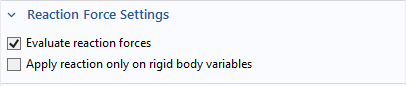
You may wonder why you need an option to get the reaction forces. The reason is that for this feature, and other similar features, there is no other way to compute the reaction forces than using Lagrange multipliers. On the other hand, always using such a formulation could potentially cause obscure problems, as will be discussed later. Thus, the need for user interaction.
Interpretation of Lagrange Multipliers
It was mentioned above that for the discrete case, the Lagrange multipliers could be directly interpreted as the nodal reaction forces. This property is much more general and not limited to finite element methods or solid mechanics. The Lagrange multipliers represent some action that is required to enforce the constraint. Often, but not always, the Lagrangian \mathcal {L } represents an energy. In such a case, Lagrange multipliers will be energetically conjugate to the constrained quantity.
The actual unit of the Lagrange multiplier also depends on the dimensionality of the object that is constrained. For solid mechanics, a boundary constrained with weak constraints will have Lagrange multipliers with the unit N/m2 = Pa. The Lagrange multiplier field can then be interpreted as the traction field that needs to be applied to the boundary in order to maintain the prescribed displacements. You should, however, not expect that field to be an accurate representation of the local stress field at the constraint. It is highly accurate in an integrated sense, though.
To illustrate the traction field for the reactions, the short cantilever beam in the figure below is studied. At the fixed end, weak constraints are used.
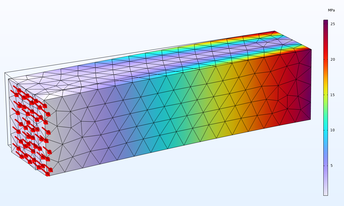 Cantilever beam with von Mises stress and applied loads.
Next, the shear stress at the constrained end is studied. According to the analytical solution, it has a parabolic distribution over the cross section. Poisson’s ratio has been chosen as zero to minimize constraint effects. In the given coordinate system, the applied load causes the shear stress σxy (and a bending normal stress σxx). Since the normal of the fixed surface is in the x direction, the traction component ty = σxy. It should thus be represented by the Lagrange multiplier for the constraint in the y direction. These results are compared in the figure below.
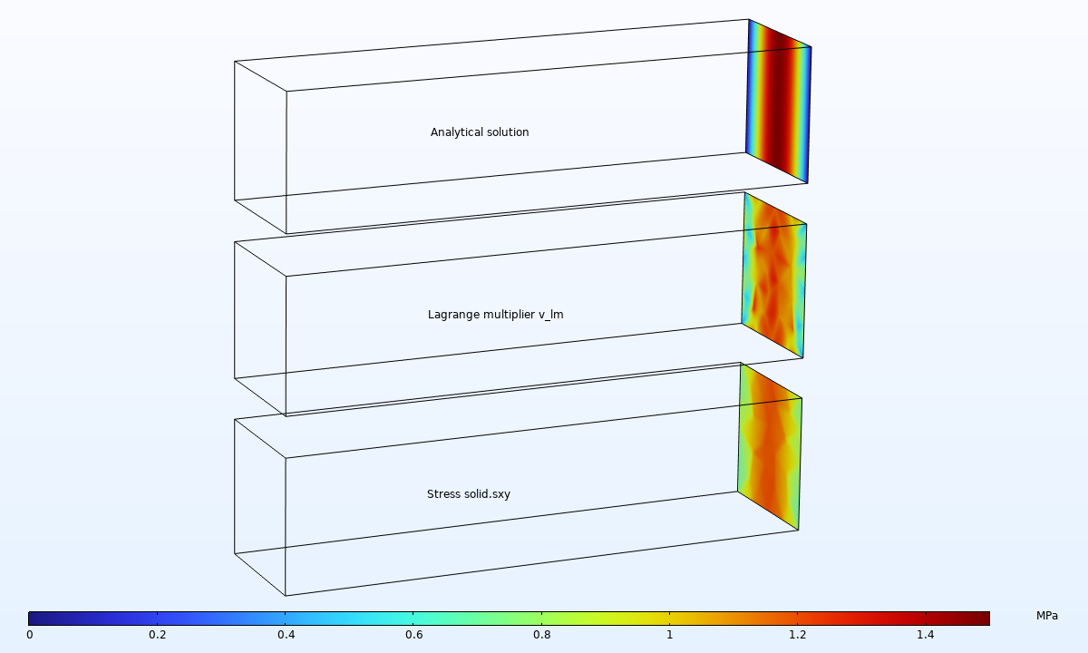 Comparison of computed shear stress, value of Lagrange multiplier, and analytical solution.
With the used mesh resolution, neither the stress nor the Lagrange multiplier provides a very accurate representation of the true solution. But there is one large difference: When integrated, the relative error in the total reaction force in the Y direction is 3% when the stress is used and 2·10-12 when the Lagrange multiplier is used.
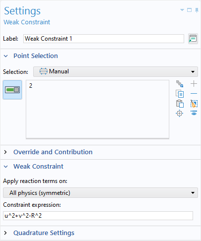
In the case that you write your own weak constraints, the values of the Lagrange multipliers may be more or less meaningful, depending on how you formulate the constraint. As an example, assume that a point should be constrained so that, after deformation, it is located somewhere on a circle with radius R around its original position.
Below, two different ways in which you could enter such a constraint are shown:

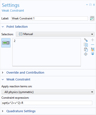
Different ways of entering the same constraint in the settings for a Weak Constraint node.
Both expressions will give the same solution with a similar number of iterations. However, in the first case, the value of the Lagrange multiplier is very difficult to interpret. From a dimensional point of view, it has the unit N/m (since it multiplies a constraint with unit m2). With the second formulation, it is actually the radial displacement that it constrained. The computed Lagrange multiplier will be the force acting on the structure from the support. The orientation of the reaction force is not obvious, but will act in the radial direction. Physically, the structure is thus supported by a frictionless circular boundary.
There are, however, two possible correct solutions to this problem. There are two places on the circle where the point may attach. This essentially represents a contact on the inside of the circle or on the outside of the circle. The solution you get depends on the initial conditions.
Things to be Aware of When Using Weak Constraints
Conflicting Constraints
The most common source of problems when using weak constraints is that they cannot coexist with the standard pointwise constraints if applied to the same DOF. Such a conflict may cause errors like “singular matrix”, “NaN or Inf found”, or even an outright erroneous solution. This is usually nothing that you want to do consciously, but it may happen inadvertently.
One example is if you use a weak constraint on one boundary, and a pointwise constraint on an adjacent boundary. Then there will be a conflict on the common edge. Usually, the easiest solution is to convert all connected constraints into the same formulation (probably weak, since there was a reason for you selecting it somewhere in the first place). Some constraints also have sections in their settings for Exclude Edges and Exclude Points. By adding the conflicting edge to such a selection, you can also resolve the problem.
In some cases, it is not obvious that a conflict can occur at all. There may be constraints that you did not think of because they were added more or less automatically. A Continuity condition is one such case.
More subtle is the situation in the Shell interface, where every node has an implicit constraint on a rotational DOF (rotation around the normal to the shell surface). Thus, if you add a weak constraint that involves rotations (say, a Fixed Constraint) to any object in a Shell interface, there will be a conflict. All rotational constraints (including the implicit ones) must then be changed into a weak formulation.
Lagrange Multiplier Units
In most cases, the Lagrange multipliers in COMSOL Multiphysics® do not carry a unit. This makes them stand out from almost all other quantities. The unit is implicit and can only be inferred from your knowledge about what the reaction field represents. If you are going to use Lagrange multipliers extensively during result evaluation, you may want to create intermediate variables where you include the unit.
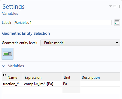
Adding a variable with a unit to represent a Lagrange multiplier field.
Variable Scaling
Sometimes, the inclusion of Lagrange multipliers will make a nonlinear problem use a lot of iterations, or even not converge. The most probable reason for this happening is that the tolerances were not handled properly. The best way to fix this and ensure the tolerances are properly handled is to perform manual scaling of the Lagrange multiplier DOFs. To do this, go to the Dependent Variables nodes in the solver sequence and add an appropriate scaling. The scale should provide the order of magnitude of the Lagrange multiplier, that is, the reaction flux that it represents.
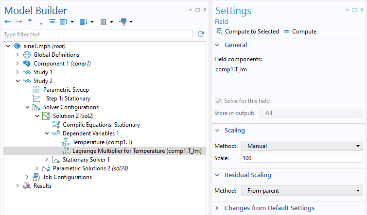 Setting a manual scale for a variable.
Iterative Solvers
If you are using an iterative solver for solving the linear system of equations, Lagrange multipliers can cause problems. There are zeros on the diagonal of the stiffness matrix, so it is no longer positive definite as it would be for most standard finite element formulations.
Because of this, certain linear solvers and preconditioners cannot be used for solving problems with weak constraints, namely the conjugate gradients iterative solver and the SOR class of preconditioners and smoothers. You can try another iterative solver and use the Vanka algorithm with the Lagrange multipliers as the Vanka variables, or use the incomplete LU factorization algorithm as a preconditioner.
For multiphysics problems, one possibility is to use a segregated approach, and if feasible due to model size, use a direct solver for the fields that involve Lagrange multipliers.
Singularity in Lagrange Multiplier DOFs
When you switch a standard constraint into being weak, it is numerically well behaved. But if you write your own nonlinear constraints, or use certain expressions for constrained variables, then it may happen that the Lagrange multiplier part of the stiffness matrix becomes singular.
The nonlinear constraint example used above, when a node is constrained to move to a circle around its original location, will actually fail in its original configuration.
The constraint expression here is actually a paraboloid centered at the node, so its gradient is zero when u = v = 0. This can easily be overcome by adding an initial condition for the displacement field.
As an alternative, you could add an artificial “stiffness” to the Lagrange multiplier DOF. In the example above, you can augment the expression to: u^2+v^2-R^2+1e-6*lm*(u^2+v^2 < 0.01*R^2)
The name of the Lagrange multiplier variable is lm. Due to the boolean expression, the extra contribution is active only for small displacements, so it will not affect the true solution. The effect is to place a small number on the diagonal of the stiffness matrix in order to avoid the initial singularity.
The same method was used in the "Weak Constraints" section of our following blog post: "How to Make Boundary Conditions Conditional in Your Simulation". There, the reason for the singularity was that only a time-varying part of a boundary had a prescribed value. On the remaining part of that boundary, the Lagrange multiplier DOFs were still present but without an equations defining them.
Further Learning
The weak constraints in COMSOL Multiphysics® are powerful modeling tools. You do, however, need some understanding of what actually goes on from a numerical perspective to be able to utilize them successfully.
If you want to read more about weak formulations, you can also check out the following blog posts:


Comments (0)