
When solving wave electromagnetics problems with either the RF or Wave Optics modules, we use the finite element method to solve the governing Maxwell’s equations. In this blog post, we will look at the various modeling, meshing, solving, and postprocessing options available to you and when you should use them.
The Governing Equation for Modeling Frequency Domain Wave Electromagnetics Problems
COMSOL Multiphysics uses the finite element method to solve for the electromagnetic fields within the modeling domains. Under the assumption that the fields vary sinusoidally in time at a known angular frequency \omega = 2 \pi f and that all material properties are linear with respect to field strength, the governing Maxwell’s equations in three dimensions reduce to:
where the material properties are \mu_r, the relative permeability; \epsilon_r, the relative permittivity; and \sigma , the electrical conductivity.
With the speed of light in vacuum, c_0, the above equation is solved for the electric field, \mathbf{E}=\mathbf{E}(x,y,z), throughout the modeling domain, where \mathbf{E} is a vector with components E_x, E_y, and E_z. All other quantities (such as magnetic fields, currents, and power flow) can be derived from the electric field. It is also possible to reformulate the above equation as an eigenvalue problem, where a model is solved for the resonant frequencies of the system, rather than the response of the system at a particular frequency.
The above equation is solved via the finite element method. For a conceptual introduction to this method, please see our blog series on the weak form, and for a more in-depth reference, which will explain the nuances related to electromagnetic wave problems, please see The Finite Element Method in Electromagnetics by Jian-Ming Jin. From the point of view of this blog post, however, we can break down the finite element method into these four steps:
- Model Set-Up: Defining the equations to solve, creating the model geometry, defining the material properties, setting up metallic and radiating boundaries, and connecting the model to other devices.
- Meshing: Discretizing the model space using finite elements.
- Solving: Solving a set of linear equations that describe the electric fields.
- Postprocessing: Extracting useful information from the computed electric fields.
Let’s now look at each one of these steps in more detail and describe the options available at each step.
Options for Modifying the Governing Equations
The governing equation shown above is the frequency domain form of Maxwell’s equations for wave-type problems in its most general form. However, this equation can be reformulated for several special cases.
Let us first consider the case of a modeling domain in which there is a known background electric field and we wish to place some object into this background field. The background field can be a linearly polarized plane wave, a Gaussian beam, or any general user-defined beam that satisfies Maxwell’s equations in free space. Placing an object into this field will perturb the field and lead to scattering of the background field. In such a situation, you can use the Scattered Field formulation, which solves the above equation, but makes the following substitution for the electric field:
where the background electric field is known and the relative field is the field that, once added to the background field, gives the total field that satisfies the governing Maxwell’s equations. Rather than solving for the total field, it is the relative field that is being solved. Note that the relative field is not the scattered field.
For an example of the usage of this Scattered Field formulation, which considers the radar scattering off of a perfectly electrically conductive sphere in a background plane wave and compares it to the analytic solution, please see our Computing the Radar Cross Section of a Perfectly Conducting Sphere tutorial model.
Next, let’s consider modeling in a 2D plane, where we solve for \mathbf{E}=\mathbf{E}(x,y) and can additionally simplify the modeling by considering an electric field that is polarized either In-Plane or Out-of-Plane. The In-Plane case will assume that E_z=0, while the Out-of-Plane case assumes that E_x=E_y=0. These simplifications reduce the size of the problem being solved, compared to solving for all three components of the electric field vector.
For modeling in the 2D axisymmetric plane, we solve for \mathbf{E}=\mathbf{E}(r,z), where the vector \mathbf{E} has the components E_r, E_\phi, and E_z. We can again simplify our modeling by considering the In-Plane and Out-of-Plane cases, which assume E_\phi=0 and E_r=E_z=0, respectively.
When using either the 2D or the 2D axisymmetric In-Plane formulations, it is also possible to specify an Out-of-Plane Wave Number. This is appropriate to use when there is a known out-of-plane propagation constant, or known number of azimuthal modes. For 2D problems, the electric field can be rewritten as:
and for 2D axisymmetric problems, the electric field can be rewritten as:
where k_z or m, the out-of-plane wave number, must be specified.
This modeling approach can greatly simplify the computational complexity for some types of models. For example, a structurally axisymmetric horn antenna will have a solution that varies in 3D but is composed of a sum of known azimuthal modes. It is possible to recover the 3D solution from a set of 2D axisymmetric analyses by solving for these out-of-plane modes at a much lower computational cost, as demonstrated in our Corrugated Circular Horn Antenna tutorial model.
Meshing Requirements and Capabilities
Whenever solving a wave electromagnetics problem, you must keep in mind the mesh resolution. Any wave-type problem must have a mesh that is fine enough to resolve the wavelengths in all media being modeled. This idea is fundamentally similar to the concept of the Nyquist frequency in signal processing: The sampling size (the finite element mesh size) must be at least less than one-half of the wavelength being resolved.
By default, COMSOL Multiphysics uses second-order elements to discretize the governing equations. A minimum of two elements per wavelength are necessary to solve the problem, but such a coarse mesh would give quite poor accuracy. At least five second-order elements per wavelength are typically used to resolve a wave propagating through a dielectric medium. First-order and third-order discretization is also available, but these are generally of more academic interest, since the second-order elements tend to be the best compromise between accuracy and memory requirements.
The meshing of domains to fulfill the minimum criterion of five elements per wavelength in each medium is now automated within the software, as shown in this video, which shows not only the meshing of different dielectric domains, but also the automated meshing of Perfectly Matched Layer domains. The new automated meshing capability will also set up an appropriate periodic mesh for problems with periodic boundary conditions, as demonstrated in this Frequency Selective Surface, Periodic Complementary Split Ring Resonator tutorial model.
With respect to the type of elements used, tetrahedral (in 3D) or triangular (in 2D) elements are preferred over hexahedral and prismatic (in 3D) or rectangular (in 2D) elements due to their lower dispersion error. This is a consequence of the fact that the maximum distance within an element is approximately the same in all directions for a tetrahedral element, but for a hexahedral element, the ratio of the shortest to the longest line that fits within a perfect cubic element is \sqrt3. This leads to greater error when resolving the phase of a wave traveling diagonally through a hexahedral element.
It is only necessary to use hexahedral, prismatic, or rectangular elements when you are meshing a perfectly matched layer or have some foreknowledge that the solution is strongly anisotropic in one or two directions. When resolving a wave that is decaying due to absorption in a material, such as a wave impinging upon a lossy medium, it is additionally necessary to manually resolve the skin depth with the finite element mesh, typically using a boundary layer mesh, as described here.
Manual meshing is still recommended, and usually needed, for cases when the material properties will vary during the simulation. For example, during an electromagnetic heating simulation, the material properties can be made functions of temperature. This possible variation in material properties should be considered before the solution, during the meshing step, as it is often more computationally expensive to remesh during the solution than to start with a mesh that is fine enough to resolve the eventual variations in the fields. This can require a manual and iterative approach to meshing and solving.
When solving over a wide frequency band, you can consider one of three options:
- Solve over the entire frequency range using a mesh that will resolve the shortest wavelength (highest frequency) case. This avoids any computational cost associated with remeshing, but you will use an overly fine mesh for the lower frequencies.
- Remesh at each frequency, using the parametric solver. This is an attractive option if your increments in frequency space are quite widely spaced, and if the meshing cost is relatively low.
- Use different meshes in different frequency bands. This will reduce the meshing cost, and keep the solution cost relatively low. It is essentially a combination of the above two approaches, but requires the most user effort.
It is difficult to determine ahead of time which of the above three options will be the most efficient for a particular model.
Regardless of the initial mesh that you use, you will also always want to perform a mesh refinement study. That is, re-run the simulation with progressively finer meshes and observe how the solution changes. As you make the mesh finer, the solution will become more accurate, but at a greater computational cost. It is also possible to use adaptive mesh refinement if your mesh is composed entirely of tetrahedral or triangular elements.
Solver Options
Once you have properly defined the problem and meshed your domains, COMSOL Multiphysics will take this information and form a system of linear equations, which are solved using either a direct or iterative solver. These solvers differ only in their memory requirements and solution time, but there are several options that can make your modeling more efficient, since 3D electromagnetics models will often require a lot of RAM to solve.
The direct solvers will require more memory than the iterative solvers. They are used for problems with periodic boundary conditions, eigenvalue problems, and for all 2D models. Problems with periodic boundary conditions do require the use of a direct solver, and the software will automatically do so in such cases.
Eigenvalue problems will solve faster when using a direct solver as compared to using an iterative solver, but will use more memory. For this reason, it can often be attractive to reformulate an eigenvalue problem as a frequency domain problem excited over a range of frequencies near the approximate resonances. By solving in the frequency domain, it is possible to use the more memory-efficient iterative solvers. However, for systems with high Q factors it becomes necessary to solve at many points in frequency space. For an example of reformulating an eigenvalue problem as a frequency domain problem, please see these examples of computing the Q factor of an RF coil and the Q factor of a Fabry-Perot cavity.
The iterative solvers used for frequency-domain simulations come with three different options defined by the Analysis Methodology settings of Robust (the default), Intermediate, or Fast, and can be changed within the physics interface settings. These different settings alter the type of iterative solver being used and the convergence tolerance. Most models will solve with any of these settings, and it can be worth comparing them to observe the differences in solution time and accuracy and choose the option most appropriate for your needs. Models that contain materials that have very large contrasts in the dielectric constants (~100:1) will need the Robust setting and may even require the use of the direct solver, if the iterative solver convergence is very slow.
Postprocessing Capabilities
Once you’ve solved your model, you will want to extract data from the computed electromagnetic fields. COMSOL Multiphysics will automatically produce a slice plot of the magnitude of the electric field, but there are many other postprocessing visualizations you can set up. Please see the Postprocessing & Visualization Handbook and our blog series on Postprocessing for guidance and to learn how to create images such as those shown below.
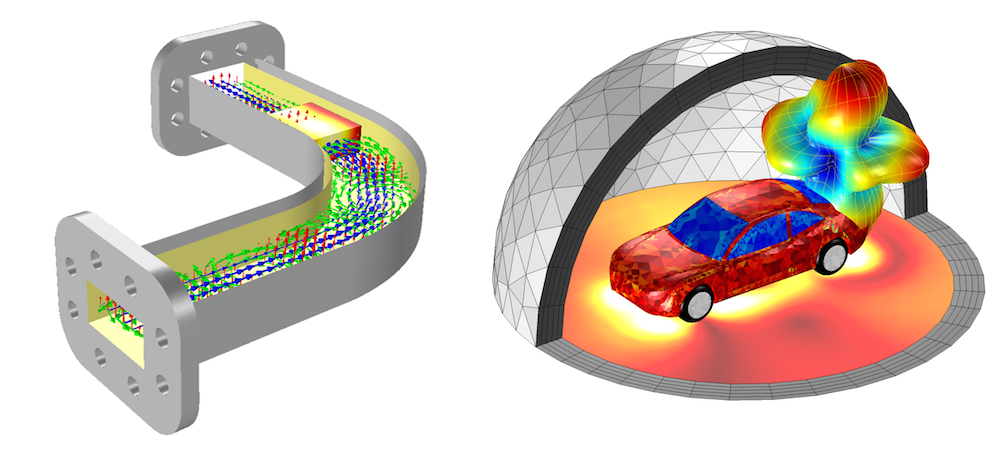
Attractive visualizations can be created by plotting combinations of the solution fields, meshes, and geometry.
Of course, good-looking images are not enough — we also want to extract numerical information from our models. COMSOL Multiphysics will automatically make available the S-parameters whenever using Ports or Lumped Ports, as well as the Lumped Port current, voltage, power, and impedance. For a model with multiple Ports or Lumped Ports, it is also possible to automatically set up a Port Sweep, as demonstrated in this tutorial model of a Ferrite Circulator, and write out a Touchstone file of the results. For eigenvalue problems, the resonant frequencies and Q factors are automatically computed.
For models of antennas or for scattered field models, it is additionally possible to compute and plot the far-field radiated pattern, the gain, and the axial ratio.
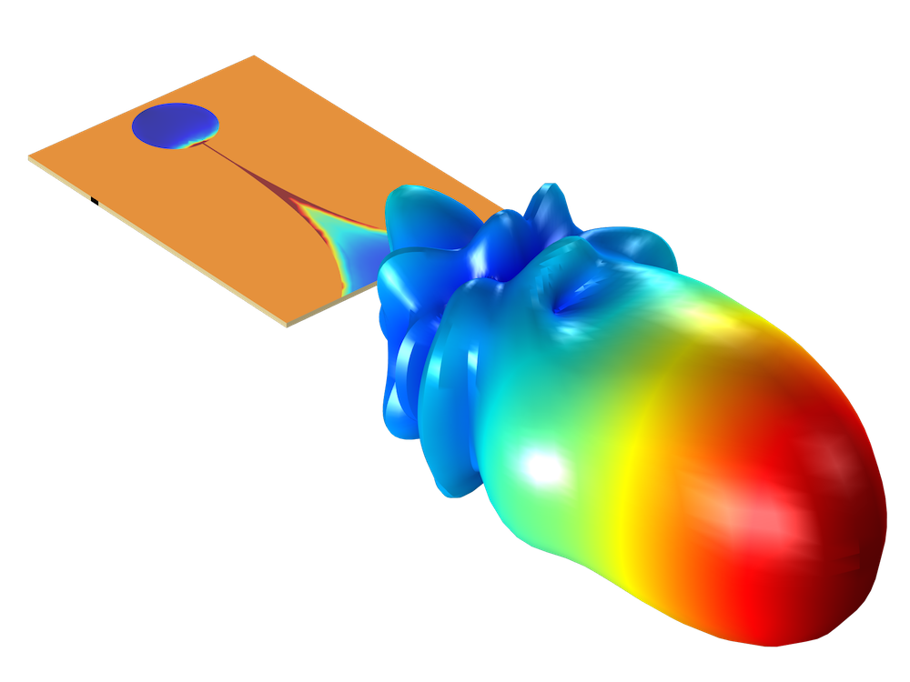
Far-field radiation pattern of a Vivaldi antenna.
You can also integrate any derived quantity over domains, boundaries, and edges to compute, for example, the heat dissipated inside of lossy materials or the total electromagnetic energy within a cavity. Of course, there is a great deal more that you can do, and here we have just looked at the most commonly used postprocessing features.
Summary of Wave Electromagnetics Simulation Tools
We’ve looked at the various different formulations of the governing frequency domain form of Maxwell’s equations as applied to solving wave electromagnetics problems and when they should be used. The meshing requirements and capabilities have been discussed as well as the options for solving your models. You should also have a broad overview of the postprocessing functionality and where to go for more information about visualizing your data in COMSOL Multiphysics.
This information, along with the previous blog posts on defining the material properties, setting up metallic and radiating boundaries, and connecting the model to other devices should now give you a reasonably complete picture of what can be done with frequency domain electromagnetic wave modeling in the RF and Wave Optics modules. The software documentation, of course, goes into greater depth about all of the features and capabilities within the software.
If you are interested in using the RF or Wave Optics modules for your modeling needs, please contact us.


Comments (0)