Modeling the Swirling Flow of a Hydrocyclone
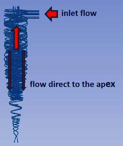
Hydrocyclones are industrial devices used as processing units in fluid and particle technology. A hydrocyclone is an apparatus consisting of a cylindrical or a cylindrical-conical body with a tangential or involute entrance to admit the fluid inside. There are also two opposite exits, the top exit which is the vortex finder and the bottom exit called apex. In a hydrocyclone the fluid and the transported particles experiment high centrifugal forces which force the former to move outward towards the solid walls and then to flow downwards to the bottom exit. On the other hand, the fluid and the particles suffer also an inwardly acting drag which can drive them towards the central region of the vessel. There, fluid and particles would travel upwards leaving the vessel through the vortex finder. These phenomena, and then the performance of a hydrocyclone, depends on the complex flow pattern which develops inside the vessel. The flow pattern results from a three dimensional turbulent swirling flow confined in the cylindrical and conical geometry of the hydrocyclone. The fluid flow is characterized by a tangential movement, known as a Rankine vortex, combination of a forced vortex and a free vortex (Fig. 1), which is completed by an axial flow in two opposite directions, one towards the apex (underflow discharge) near the walls and a reverse flow travelling to the vortex finder (overflow discharge) near the center of the hydrocyclone. Furthermore, the radial component of velocity plays an important role in the operation of a hydrocyclone, although it is one order of magnitude smaller than the other two components, as shown by experimental and theoretical studies. The 3D character of the flow and the anisotropy of its turbulence make difficult and computationally intensive the simulation of the flow in hydrocyclones. In this work we have improved a previous work and developed a new 3D model of the swirling flow in a conical hydrocyclone by using the CFD module of COMSOL Multiphysics®. Turbulence is modeled by using the Reynolds-Averaged Navier-Stokes equations and the v-2f turbulence closure. The results of the simulations are very satisfactory, being able to reproduce the general flow pattern. Finally, the computed velocity profiles are compared with laser Doppler measurements of axial and tangential velocities made by the some authors, in order to assess its goodness.

Download
- chine__presentation.pdf - 0.85MB
- chine__paper.pdf - 0.37MB
- chine__abstract.pdf - 0.07MB


