Finite Element Time-Dependent Analysis
In Part 1 of this course, we discussed the applicability of frequency-domain and time-dependent analyses. Let's recap the circumstances that require a transient model:
- The excitation is a short pulse or includes more than one frequency component.
- The problem becomes nonlinear. The nonlinearity can be due to large signal excitation and higher harmonic generation, a nonlinear magnetization model, or a geometry/topology change because of large deformation.
- The output of interest is the transient response to an excitation.
In this part of the course, we use the same dynamic speaker driver as in Part 2 (which focuses on a frequency-domain study) to discuss the specific considerations for running a nonlinear transient analysis. The model is solved in the 2D axisymmetric space dimension, and the focuses of this study are to characterize the nonlinear behavior of the driver due to large deformation of the moving parts and to determine the total harmonic distortion (THD) of the acoustic signals produced by the system.
This analysis requires a moving mesh in the deforming fluid domains around the moving parts, together with transient acoustic formulations. An important consideration when modeling acoustics in moving domains is that the moving mesh functionality is only compatible with first-order-in-time formulations. Consequently, deforming fluid domains must use Thermoviscous Acoustics, which is first order in time, rather than Pressure Acoustics, which is second order in time. Fluid domains farther away from the moving parts, where mesh deformation is not required, can still be modeled using pressure acoustics. These considerations are discussed in detail in this section.
Geometry
The highlighted air volume is constructed as a layered computational domain, with an inner region for the moving mesh and near-boundary thermoviscous acoustic effects, a surrounding pressure acoustics region for wave propagation, and an outer Perfectly Matched Layer (PML) to suppress unphysical reflections from the artificial boundaries of the finite computational domain. The Perfectly Matched Boundaryfeature used in Part 2 is only available in a frequency-domain pressure acoustics model. For time-domain simulations, use the Perfectly Matched Layer feature, which is applied to a virtual domain attached to an open boundary.
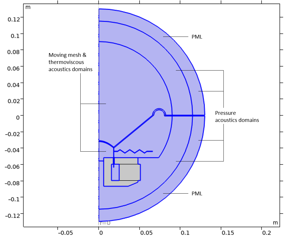
The geometry for a transient analysis. There are distinct fluid domains for moving mesh and thermoviscous acoustics, pressure acoustics, and a PML to absorb outgoing waves.
The geometrical thickness of the perfectly matched layer (PML) in a geometry needs to be set adequately. The thickness can be determined by the following two meshing considerations:
- Use the same mesh element size as that in the adjacent physical domain
- Use a structured mesh with at least 6 mesh layers for the rational scaling and 8 for the polynomial scaling
The recommendation of using the same mesh size in both physical and PML regions is because of the implementation of PML in the time domain: There is no stretching with respect to the real coordinate in the PML, thus, the waves propagate through the PML with the same wavelength that they have in the physical region.
Required Physics Interfaces
Performing the transient analysis requires the Magnetic Fields interface from the AC/DC Module; and the Solid Mechanics, Pressure Acoustics, Transient, and Thermoviscous Acoustics, Transient interfaces from the Acoustics Module. In addition, a moving mesh is required to capture the back EMF and nonlinear effects caused by changes in geometry.
The Necessity of Using a Moving Mesh in Transient Studies
The Lorentz Coupling feature, available as an option in the built-in Magnetomechanics, Solid multiphysics coupling, is formulated differently for transient analysis than for frequency-domain analysis.
In the frequency domain, the formulation explicitly includes the back EMF contributions: It passes the Lorentz force from the Magnetic Fields interface to the Solid Mechanics interface and passes the structural velocity that leads to the induced electric field from the Solid Mechanics interface to the Magnetic Fields interface. However, in the time domain, only the Lorentz force is passed from the Magnetic Fields interface to the Solid Mechanics interface, but the induced currents are not included in the formulation. You need to use a moving mesh in order to capture the back EMF contributions. This specific handling of transient analysis is to avoid double counting of the back EMF when one wants to use a moving mesh to capture nonlinearity due to large deformations and geometry/topology changes, like when the coil is moving partially or fully in and out of the magnetic gap. Since the induced currents are captured automatically by a moving mesh, including them in the coupling formulation will give wrong results.
Therefore, in transient studies it is always necessary to use a moving mesh even for small displacements, because the induced currents are only captured that way. In the current case, we are also interested in modeling the effect of structure deformations on the magnetic field and acoustic field, which adds another source of nonlinearity to the problem .
Adding the Required Physics Interfaces
The most convenient way to add all the required physics is to select the Magnetomechanics, Solid, Thermoviscous Acoustics, Transient, and Pressure Acoustics, Transient interfaces at the Select Physics step.
The Magnetomechanics, Solid interface is available under Structural Mechanics > Electromagnetics-Structure Interaction > Magnetomechanics in the Select Physics window of the Model Wizard. This multiphysics interface combines the Solid Mechanics and Magnetic Fields interfaces with moving mesh functionality. When it is added, these physics interfaces are inserted automatically, along with the Magnetomechanics, Solid multiphysics coupling, as shown in the image below.
 The Select Physics window of the Model Wizard with the Structural Mechanics node expanded. The Magnetomechanics, Solid physics interface is selected.
The Magnetomechanics, Solid interface is under Structural Mechanics > Electromagnetics-Structure Interaction > Magnetomechanics in the Select Physics window of the Model Wizard.
Next, add the acoustic interfaces. Note that COMSOL provides distinct physics interfaces for solving specific wave-equation formulations in fluids for frequency-domain and time-domain analyses. It is therefore important to select the physics interface that matches the intended study type. The following images show the location of the transient Pressure Acoustics and Thermoviscous Acoustics interfaces in the Select Physics window of the Model Wizard.
 The Select Physics window of the Model Wizard with the Pressure Acoustics node expanded. The Pressure Acoustics, Transient physics interface is selected.
The Pressure Acoustics, Transient interface is under Acoustics > Pressure Acoustic in the Select Physics window of the Model Wizard.
 The Select Physics window of the Model Wizard with the Thermoviscous node expanded. The Thermoviscous Acoustic, Transient physics interface is selected.
The Thermoviscous Acoustics, Transient interface is under Acoustics > Thermoviscous Acoustic in the Select Physics window of the Model Wizard.
Later, additional multiphysics couplings can be manually added under the Multiphysics node in the model tree to connect the solid and fluid domains and enforce continuity between the pressure acoustics and thermoviscous acoustics regions.
Domain Selections for the Physics Interfaces
As a best practice, begin by creating domain selections for each physics interface to keep the model organized and simplify the setup process. In the frequency-domain analysis in Part 2, these selections were created under the Geometry node. Here, they are created under the Definitions node within the component, as shown in the images below.
 The Magnetic Fields node selected in the Model Builder window and the Settings window showing the Input Entities section with the corresponding selected domain highlighted in blue in the graphics window.
Domain selection for the Magnetic Fields interface.
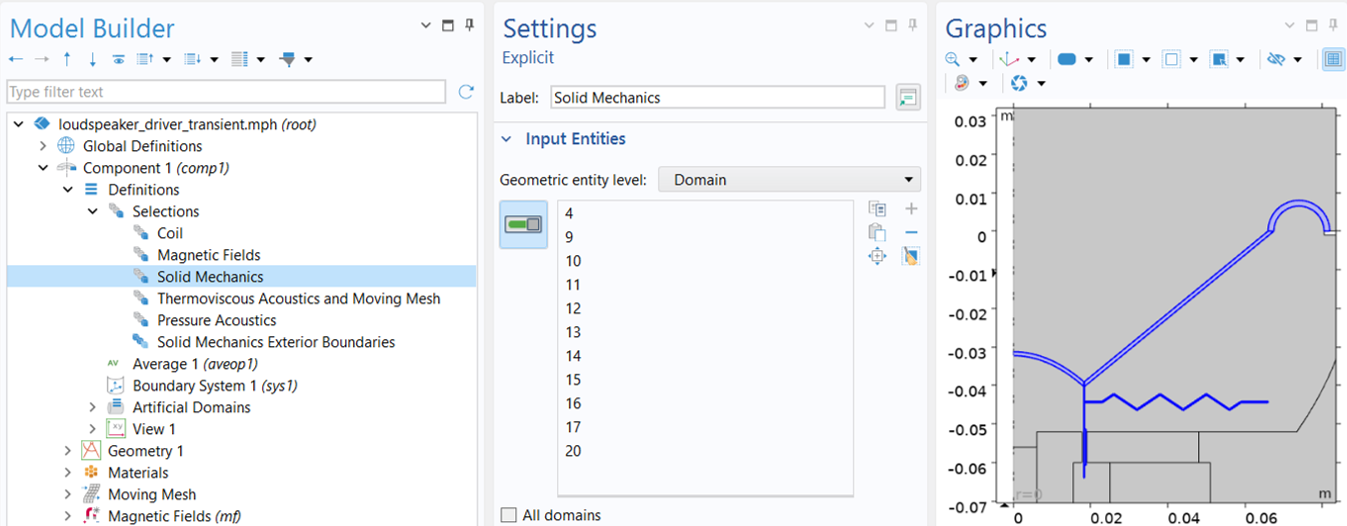 The domain selection settings window for the Solid Mechanics interface with the selected domains highlighed in blue in the graphics window.
Domain selection for the Solid Mechanics interface.
 The domain selection settings window for the Thermoviscous Acoustics and Moving Mesh interface with the selected domains highlighed in blue in the graphics window.
Domain selection for the Thermoviscous Acoustics and Moving Mesh interfaces.
 The domain selection settings window for the Pressure Acoustics interface with the selected geometry highlighed in blue in the graphics window.
Domain selection for the Pressure Acoustics interface.
The Magnetic Fields domains encompass the regions beneath the diaphragm, including all electromagnetic components—the magnet, soft iron pole piece, top plate, coil, and former—as well as the spider and the air domain below the cone. The Solid Mechanics domains comprise all moving parts: the coil, former, cone, spider, and surround. The Thermoviscous Acoustics and Moving Mesh domains consist of the air regions adjacent to the moving solids, while the Pressure Acoustics domains cover the remaining air regions farther from the moving parts.
The resulting selections are then assigned to the Domain Selection setting at the main node of each physics interface.
Setting Up the Physics
Moving Mesh
As discussed earlier, using a moving mesh is essential for capturing the back EMF in transient analysis with the Lorentz Coupling feature. It is also required to account for the effects of geometry changes caused by large deformations on physics interfaces formulated in the spatial frame, such as Magnetic Fields and Thermoviscous Acoustics, Transient. These effects contribute to the nonlinear behavior of the system and are therefore critical for distortion analysis.
The following steps are necessary in order to set up the moving mesh correctly:
1) In the Deforming Domain 1 subnode, select Thermoviscous Acoustics and Moving Mesh for Domain Selection and choose Laplace from the Mesh smoothing type list for Smoothing, as seen in the image below. Once the deforming domains are specified, prescribed mesh displacements using the solid displacement components are automatically added to all boundaries next to a solid, and a fixed boundary is used for all other outer boundaries.
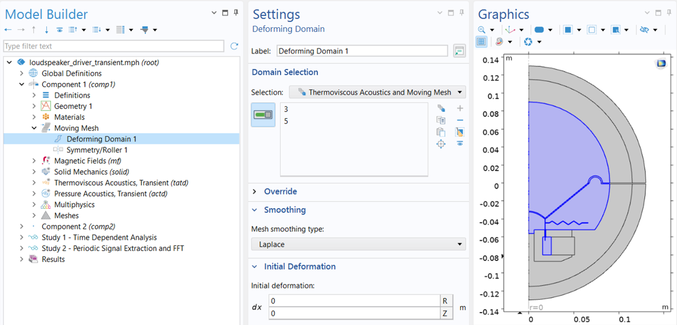 The COMSOL Multiphysics UI showing the Model Builder with the Deforming Domain feature selected and the corresponding Settings window with Laplace selected for the mesh smoothing type.
The Laplace mesh smoothing type is used in the deforming domains.
Compared to other nonlinear smoothing methods, the Laplace smoothing is the cheapest option in terms of computations because it is linear and uses one equation for each coordinate direction, which are not coupled together. This method is suitable when the mesh deformation is not too large, and especially when it is used together with an Automatic Remeshing feature, which ensures a new mesh is created whenever the mesh quality becomes less than a given limit.
2) In the Symmetry/Roller 1 subnode, select the boundaries at r = 0 for the Boundary Selection. This allows the mesh to "slide" there.
 The COMSOL Multiphysics UI with the Symmetry/Roller feature selected and the corresponding settings and model.
The Symmetry/Roller condition is applied to boundaries lying at r = 0.
Perfectly Matched Layer
When the Pressure Acoustics, Transient interface is present in the model, a Perfectly Matched Layer node becomes available under Component 1 > Definitions > Artificial Domains. In its settings window, select the two outermost domains under Domain Selection, then set the Type field to Spherical in the Geometry section.
In the Scaling section, keep the default Polynomial option for Coordinate stretching type, and ensure that Typical wavelength from is set to use the Pressure Acoustics, Transient physics interface.
For the Polynomial stretching type, the recommended values for the PML scaling factor and scaling curvature parameter are 1 and 3, respectively. If the Rational stretching type is used instead, the recommended values are 1 and 1.
 The COMSOL Multiphysics UI showing the Model Builder with the Perfectly Matched Layer feature selected, the corresponding settings, and the geometry with the outer layer highlighted in blue to show where the PML feature is applied.
The Perfectly Matched Layer settings for the transient analysis.
Magnetic Fields
The Magnetic Fields physics is configured in much the same way as in the frequency-domain analysis, except that a time-dependent voltage signal, V(t), is applied to the voice coil for the transient analysis. The choice of a specific type of input signal depends on the characteristic under investigation. In this case, the input is a harmonic voltage signal:

The input signal frequency and the amplitude are chosen as f0=70Hz and V0=10V, respectively.
When solving a transient model, it is good practice to ramp up the load to minimize numerical error. An instantaneously applied load leads to a lot of high-frequency content generation due to the inertia effect of the system it applies to, and when they are unresolved, numerical error or even solver divergence can occur. This is also physically motivated since most loads cannot truly change instantaneously in time. You can use a Step or Ramp function with appropriate smoothing for this purpose.
In this analysis, we use the driving signal period, T0=1/f0, to define a ramp function, rm1(t), that has a slope of 1/T0 . The ramped input signal, V0 *sin(2πf0t)*rm1(t), is then used to define the coil voltage, as shown in the image below. This allows the load to take one period to reach its full magnitude.
 The Ramp function selected in the Model Builder, the corresponding Parameters and Smoothing settings, and the function plot.
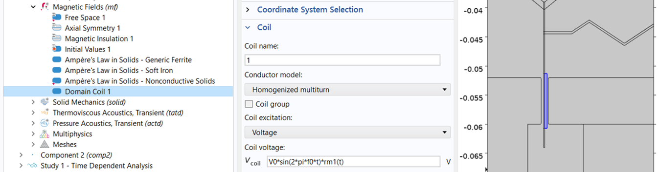 A close-up of the Coil feature selected in the Model Builder and the Coil section of the corresponding Settings window, with a close-up of the model in the Graphics window.
A Ramp function is defined using the driving signal period (top), and is then used to smooth the input signal (bottom).
Solid Mechanics
Compared to the frequency-domain analysis, the main difference in the Solid Mechanics setup for transient analysis is the choice of mechanical damping model. Note that loss factor damping is applicable only to frequency-domain analyses. For transient analyses, use one of the damping models that are supported in the time domain, such as Rayleigh damping, Viscous damping, or Wave attenuation.
Here, the losses in the spider and surround are modeled using Rayleigh damping, consistent with the damping approach used in the frequency-domain study in Part 2. For the former and cone that used Isotropic loss factor in the frequency-domain study, Viscous damping is used instead in the transient analysis, with the damping parameters defined as shown below.
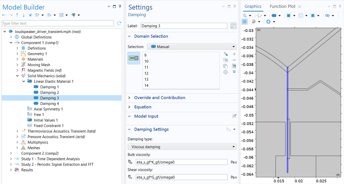 The Damping 3 mode selected in the Model Builder and the Settings window with Viscous damping setting selected for the glass-fiber former, which is shown in blue in the graphics window.
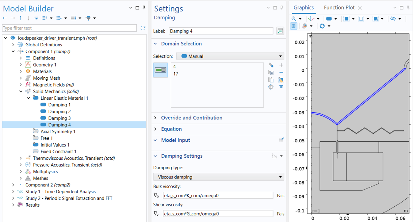 The Damping 4 selected in the Model Builder and the Settings window with Viscous damping setting selected for the composite-paper cone, which is shown in blue, in the graphics window.
Viscous damping is used to model mechanical loss in the glass-fiber former (top) and composite-paper cone (bottom).
The damping parameters, bulk viscosity ( ) and Shear viscosity (
 ), are calculated from isotropic loss factor (
 ) using
 ,

where  is the driving angular frequency, and K and G are the bulk and shear moduli, respectively.
The corresponding material parameters are denoted by eta_s_gf, K_gf, and G_gf for the glass-fiber former, and eta_s_com, K_com, and G_com for the composite-paper cone, corresponding to the isotropic loss factor, bulk modulus, and shear modulus, respectively. All of these parameters, along with the angular frequency, omega_0, are defined in the Parametersnode under Global Definitions.
Thermoviscous Acoustics, Transient
As mentioned earlier, thermoviscous acoustics should be used to model acoustics in moving domains because its first-order-in-time formulation is compatible with the moving mesh functionality. Compared with pressure acoustics, which solves only for the acoustic pressure, thermoviscous acoustics solves for pressure, particle velocity, and temperature variation, making it computationally more expensive. When thermal conduction losses are negligible, an adiabatic formulation is often preferable because it avoids solving for the temperature field while still accounting for viscous effects where needed, thereby helping to reduce the computational cost.
The adiabatic formulation can be activated by selecting the Adiabatic formulation checkbox in the Thermoviscous Acoustics Equation Settings section of the Thermoviscous Acoustics, Transient interface settings window, as shown below. Also, under the Transient Solver and Mesh Settings section, enter Nhar*f0 in the Maximum frequency to resolve field. This ensures that the autogenerated time-dependent solver uses time steps small enough to resolve the highest frequency the model needs to capture. In this case, Nhar, the parameter that defines the number of harmonics to resolve, has a value of 3 and is defined under the Parameters node under Global Definitions.
The Time stepping setting in the same section enables you to set the time-stepping method as either Fixed (preferred) or Free. In this case, it is recommended that you use the default Fixed (preferred) method, which is best suited for handling wave propagation.
 The Thermoviscous Acoustics, Transient settings window with the Adiabatic formulations checkbox selected for the Thermoviscous Acoustics Equation Settings. The graphics window to the right of the settings window highlights the thermoviscous domain selections in blue.
Adiabatic formulation of thermoviscous acoustics is selected to reduce computation cost.
The default wall condition in thermoviscous acoustics is No Slip. When combined with a sufficiently fine boundary-layer mesh, this condition accurately resolves viscous losses near walls. In this model, the No Slip condition is applied only to boundaries adjacent to the narrow magnetic air gap, where thermoviscous losses are significant. For walls adjacent to larger fluid domains, Slip (perfect) is used instead, avoiding the need for extremely fine boundary-layer meshes in regions where thermoviscous losses are negligible. This reduces memory requirements and solution time without compromising accuracy. With adiabatic thermal conditions, the Slip (perfect) formulation is physically equivalent to pressure acoustics.
This is implemented by changing the Mechanical condition in the default Wall 1 node from No Slip to Slip (perfect), as shown below. A second wall node, Wall 2, is then added, where the boundaries corresponding to the narrow magnetic air gap are selected and assigned the No Slip condition.
 The Thermoviscous Acoustics, Transient (tatd) node Wall 1 selected in the Model Builder and the Settings window with the Boundary Selection and Mechanical sections expanded to define the wall conditions. The selected boundaries are shown in the graphics window in blue. The Mechanical Condition is Slip (perfect).
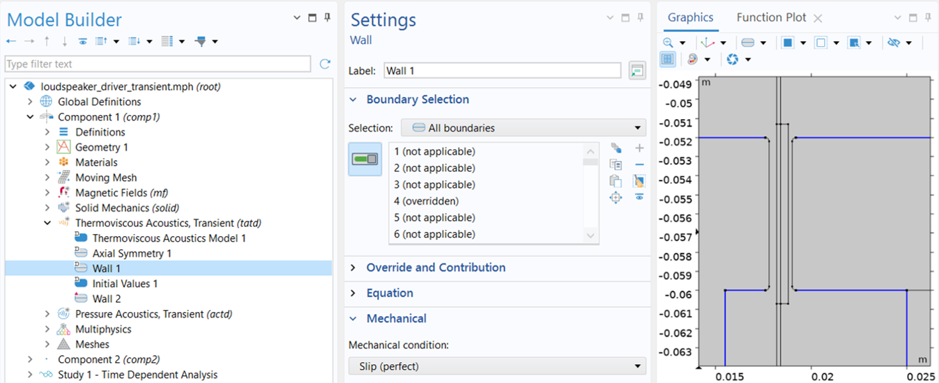 The Thermoviscous Acoustics, Transient (tatd) node Wall 2 settings window with the Boundary Selection and Mechanical sections expanded to define the wall conditions. The selected boundaries are shown in the Graphics window in blue. The Mechanical Condition is No slip.
The No Slip wall condition is applied only to the boundaries of the narrow magnetic air gap (bottom), while all other walls are assigned the Slip condition (top).
As a result, the use of thermoviscous acoustics not only accommodates the moving mesh but also naturally captures the viscous damping that is important in the narrow magnetic air gap between the pole pieces and the voice coil. In the frequency-domain analysis in Part 2, the same effect is instead accounted for using the Narrow Region Acoustics feature, which is available only in the frequency domain.
Pressure Acoustics, Transient
The remaining air domains, including the two Perfectly Matched Layer domains, are modeled using the Pressure Acoustics, Transient interface. The Transient Solver and Mesh Settings are configured in the same way as in the Thermoviscous Acoustics, Transient interface. This is again necessary to ensure that the autogenerated time-dependent solver uses the appropriate time step for wave propagation. When this setting is present in multiple physics interfaces, COMSOL Multiphysics determines the required time step for each interface and uses the smallest value.
 Pressure Acoustics, Transient, settings window with the Domain Selection, and the Transient Solver and Mech Settings sections expanded. The selected domains are highlighted in blue in the Graphics window.
The Pressure Acoustics, Transient physics interface settings.
Setting up Multiphysics Couplings
The next step is to set up the necessary multiphysics couplings, including the magnetics–structure, acoustic–structure, and pressure acoustics–thermoviscous acoustics couplings.
Magnetics-Structure Coupling
The Magnetic Fields and Solid Mechanics interfaces are coupled through the Magnetomechanics, Solid multiphysics coupling. As in the frequency-domain analysis, select Only use Lorentz force under the Lorentz Coupling section, since the moving-coil transducer is driven primarily by the Lorentz force. The coupling computes the Lorentz force acting on the voice coil while accounting for the magnetic field in the deformed geometry as the mesh moves.
 Magnetomechanics, Solid settings window with the Domain Selection, Coupled Interfaces, and Lorentz Coupling sections expanded. The domain selection is shown in blue in the Graphics window. The coupled interfaces are Solid Mechanics and Magnetic Fields. The checkbox is selected for Only use Lorentz force.
The Magnetomechanics, Solid coupling between the Magnetic Fields and Solid Mechanics interfaces.
Acoustic-Structure Coupling
The deforming acoustic domains are coupled to the vibrating structures at the fluid–solid interfaces through the Thermoviscous Acoustics–Structure Boundary multiphysics coupling. Similar to the Wall condition in the Thermoviscous Acoustics interface, the mechanical condition can be set to either No Slip, which enforces velocity continuity in all directions, or Slip (perfect), which enforces continuity only in the normal direction. As before, No Slip is used only on surfaces within the narrow magnetic air gap to capture the significant thermoviscous losses there, while Slip (perfect) is used on surfaces adjacent to larger air domains to reduce computational cost.
The Thermoviscous Acoustic-Stucture Boundary 1 selected in the Model Builder and the Settings window with the Boundary Selection, Equation, Coupled Interfaces, and Mechanical sections expanded. The boundary selections are highlighted in blue in the graphics window. The coupled interfaces are Thermoviscous Acoustics, Transient (tatd) and Solid Mechanics. The mechanical condition is defined as Slip (perfect).
 The Thermoviscous Acoustic-Structure Boundary 2 selected in the Model Builder and the Settings window revealing the Boundary Selection, time dependent analysis, Coupled Interfaces, and no slip mechanical condition. Boundaries 19 and 42 are selected and shown in blue in the graphics window. The coupled interfaces are Thermoviscous Acoustics, transient (tatd) and Solid Mechanics.
The Thermoviscous Acoustic–Structure Boundary coupling between the Thermoviscous Acoustics, Transient and Solid Mechanics interfaces, with Slip (perfect) applied to surfaces adjacent to large fluid domains (top) and No slip applied to surfaces within the narrow air gap (bottom).
Pressure Acoustics–Thermoviscous Acoustics Coupling
The Acoustic–Thermoviscous Acoustic Boundary coupling is used to ensure continuity on boundaries connecting pressure acoustics and thermoviscous acoustics. The coupling enforces continuity of the total normal stress as the dynamic condition and continuity of the total normal acceleration as the kinematic condition. An adiabatic condition is imposed on the total temperature to ensure consistency with the assumptions of the pressure acoustics formulation.
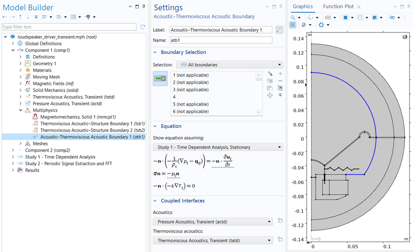 The Acoustic-Thermoviscous Boundary settings window showing the boundary selection, highlighted in blue in the graphics window. The Coupled interfaces settings show the pressure Accoustics, Transient (actd) selected for the Acoustics interface and the Thermoviscous, Transient is selected for the Thermoviscous acoustics interface.
The Acoustic-Thermoviscous Acoustic Boundary coupling between thePressure Acoustics, Transient and Thermoviscous Acoustics, Transient interfaces.
Note that this coupling should be applied at a common boundary between pressure acoustics and thermoviscous acoustics only when Slip (perfect) and adiabatic conditions are used on the thermoviscous side, as is the case here. This ensures that the boundary conditions on both sides are physically consistent. Because the coupling assumes adiabatic behavior and transfers only the normal stress, using it with No slip and isothermal conditions on the thermoviscous side would lead to an inconsistent physical representation and introduce errors.
Study Steps
Similar to the frequency-domain analysis, the transient study is also carried out using two study steps. First, a Stationary step is used to solve only the electromagnetic part of the problem in order to evaluate the field of the permanent magnet, with the driver in standstill. Then, the full Time Dependent study step takes care of all the relevant multiphysics interactions of the moving speaker.
 The Stationary Study selected in the Model Builder and the corresponding Settings window showing the tables in the Physics and Variables Selection setting.
 The Time Dependent study selected in the Model Builder and the corresponding Settings window showing settings such as the output times and physics and variables selection.
Study step settings for transient analysis.
The Time Dependent study step solves for the period of time from 0 to T_end = 4T0. The full output time range is split into two subintervals: from 0 to 3T0 and from 3T0 to T_end. The second subinterval is of the most interest since it is assumed that the steady state takes place from time 3T0. Therefore, the output time stepping is finer over the second subinterval in order to obtain a steady-state solution with better time resolution.
Automatic Remeshing
Because the mesh deforms continuously with the moving domains, its quality can deteriorate as the simulation progresses. The Automatic Remeshing option is therefore enabled in the time-dependent study to maintain satisfactory mesh quality throughout the simulation. When the mesh distortion exceeds a specified criterion, the domain is automatically remeshed, preventing highly distorted elements that could otherwise degrade numerical accuracy or lead to an ill-posed problem.
 A close-up of the Time Dependent study selected in the Model Builder and the Study Extensions settings in the corresponding Settings window.
The Automatic remeshing option is enabled in the Study Extensions section of the Time Dependent study Settings window.
Here are the steps for specifying the condition for remeshing:
1) Click Show Default Solver in the Study toolbar.
2) Expand the solver sequence and click Automatic Remeshing under the Time-Dependent Solver 1 node.
3) In the Condition for Remeshing section of the Settings window for Automatic Remeshing, choose Distortion for the Condition type and enter 2.5 in the Stop when distortion exceeds text field.
4) In the Remesh section, clear the Store solution when new meshes are created checkbox, as seen in the image below.
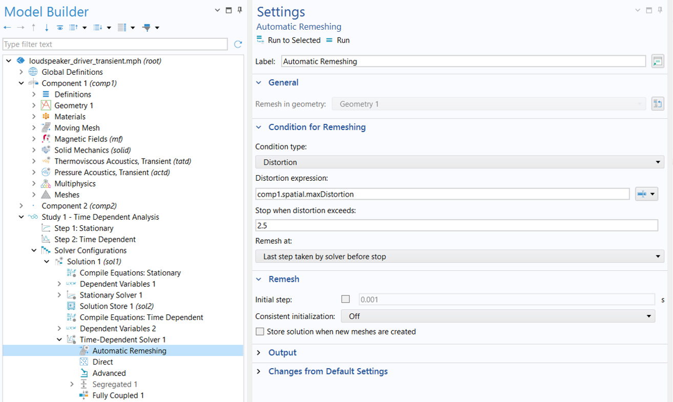 The Automatic Remeshing feature selected in the Model Builder and the corresponding Settings window showing the Condition for Remeshing settings, such as Distortion set as the condition type.
The Condition for Remeshing setup.
These settings ensure that remeshing is triggered when the maximum element distortion in the deforming domains, stored in the variable named comp1.spatial.maxDistortion, becomes larger than 2.5. In addition, the solver stores solutions and deformed configurations only for time intervals containing the requested output times, rather than for every newly generated mesh.
Time-Dependent Solver
With automatic remeshing enabled, we need to make a few changes to the default time-dependent solver settings:
1) Change the scale for the Spatial Mesh Displacement variable to 1e-4, which is smaller than the default value. Using a smaller scalemakes the solver apply a stricter convergence criterion to the mesh motion. This can improve accuracy when the expected mesh displacement is small, ensuring that small changes in the moving geometry are adequately resolved. To modify the scale, expand Study 1 > Solver Configurations > Solution 1 (sol1) > Dependent Variables 2, select Spatial Mesh Displacement (comp1.spatial.disp), and locate the Scaling section, as shown below.
 The Spatial Mesh Displacement node, under the dependent variables solver configurations, settings window with the Scaling set to 1e-4.
A smaller scale for theSpatial Mesh Displacement variable improves the solver's resolution of small mesh motions.
2) The default Time-Dependent Solver is optimized for analyses without remeshing. It uses Generalized alpha for Time Stepping, together with a manual time step determined by the Maximum frequency to resolve settings in the physics interfaces to adequately resolve the highest specified frequency component.
When Automatic Remeshing is used, change the Time Stepping method to BDF, which provides more robust event detection for triggering remeshing. However, the default time-step criterion for resolving the acoustic waves should be retained. To do this, set Steps taken by solver to Manual and keep the default expression, min(1/(60*Nhar*f0),1/(60*Nhar*f0)), in the Time step field. This expression selects the smaller of the time steps required to resolve the maximum frequencies specified in the Thermoviscous Acoustics, Transient and Pressure Acoustics, Transient interfaces.
Lastly, in the Time Stepping section, keep the BDF order at its default value of 2, but use smaller-than-default values for both Initial step fraction and Initial step growth rate , set here to 0.5 and 1.4, respectively, to provide a more gradual solver startup. This reduces the initial time step and slows its progression toward the prescribed time step, improving numerical stability and accuracy during the initial transient, when the BDF method operates at a lower order. The final Time Stepping settings are shown in the figure below.
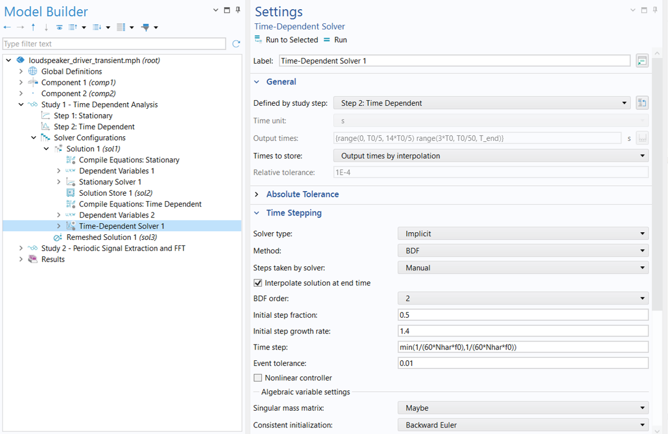 The Time-Dependent Solver selected in the Model Builder and a close-up of the Time Stepping settings in the corresponding Settings window.
Time Stepping settings for the Time-Dependent Solver.
As also shown in the figure above, one additional change is made in the General section of the Time-Dependent Solver settings, located above the Time Stepping section. Set Times to store to Output times by interpolation so that solutions at the requested output times are obtained by interpolation from the solver’s internal time steps.
3) By default, the MUMPS direct solver is used to solve the system at each time step. In this case, we instead use PARDISO, which can provide better computational performance and memory efficiency for the large, fully coupled linear systems arising in this model. Another option is the NVIDIA CUDA® Direct Sparse Solver (NVIDIA cuDSS), which can be used with a compatible NVIDIA GPU to further accelerate computations.
 The Model Builder with the Direct node selected under the Time-Dependent Solver and the Settings window with PARDISO selected for the solver.
PARDISO direct solver is used to solve the problem at each time step.
4) The default solver uses a segregated approach, solving the Spatial Mesh Displacement separately from the other dependent variables to reduce memory usage. In this model, however, the mesh motion is strongly coupled to the physical fields, so a Fully Coupled approach is used instead to solve all dependent variables simultaneously, improving solver robustness and convergence. To make this change, right-click the Time-Dependent Solver 1 node and choose Fully Coupled.
Two additional adjustments to the Fully Coupled solver are necessary to improve solver converge. In the Method and Termination section, set the Nonlinear method to Automatic (Newton) , allowing the solver to automatically select an appropriate Newton strategy for robust convergence. Also, increase the Maximum number of iterations to 10 to provide sufficient nonlinear iterations for the strongly coupled moving-mesh problem to converge at each time step.
 The Model Builder with the Fully Coupled node selected under Time-Dependent Solver and the Settings window with General and Method and Termination sections expanded.
This strongly coupled moving-mesh problem requires a fully coupled approach.
Note that the solver adjustments described above are specific to this highly nonlinear problem, which involves both a moving mesh and automatic remeshing. Such solver modifications are not generally required. For most problems without remeshing, the autogenerated solver settings provide a robust starting point and can typically be used without modification.
Initial Mesh
We need an initial mesh to start with, and a new mesh will be automatically generated whenever the mesh distortion tolerance is reached.
For transient models, the mesh needs to be able to resolve the maximal frequency you want to capture, say fmax. This frequency translates to a minimal wavelength, λmin = c/fmax, and in turn to a maximum element size, hmax < λmin/5. Use this criteria to determine the maximum element size for each domain.
The initial mesh is seen in the image below. It uses Mapped meshes for the thin solid domains, including the coil, former, spider, cone, and suspension, and Free Triangular meshes for the rest of the physical domains. Mapped meshes with a distribution of 8 elements are applied to discretize the PML domains. Refer to the attached MPH-file for the detailed meshing sequence.
 A close-up of the initial mesh and the mesh of the half-circle.
The initial mesh used for the transient analysis.
The present model runs at a relatively low frequency (including the harmonics) and does not require a resolution of eddy currents (the skin depth) in the top plate and pole piece. Thus, compared to the frequency-domain analysis, the boundary layer meshes in those iron domains have been removed.
Transient Solutions and Analysis
The animation below shows the magnetic field in and around the voice coil gap, the motion of the voice coil (orange), the former, the spider, and the cone (pink), as well as how the moving mesh adapts the mesh to the changed topology of the system during the time period of 3T0 to 4T0.
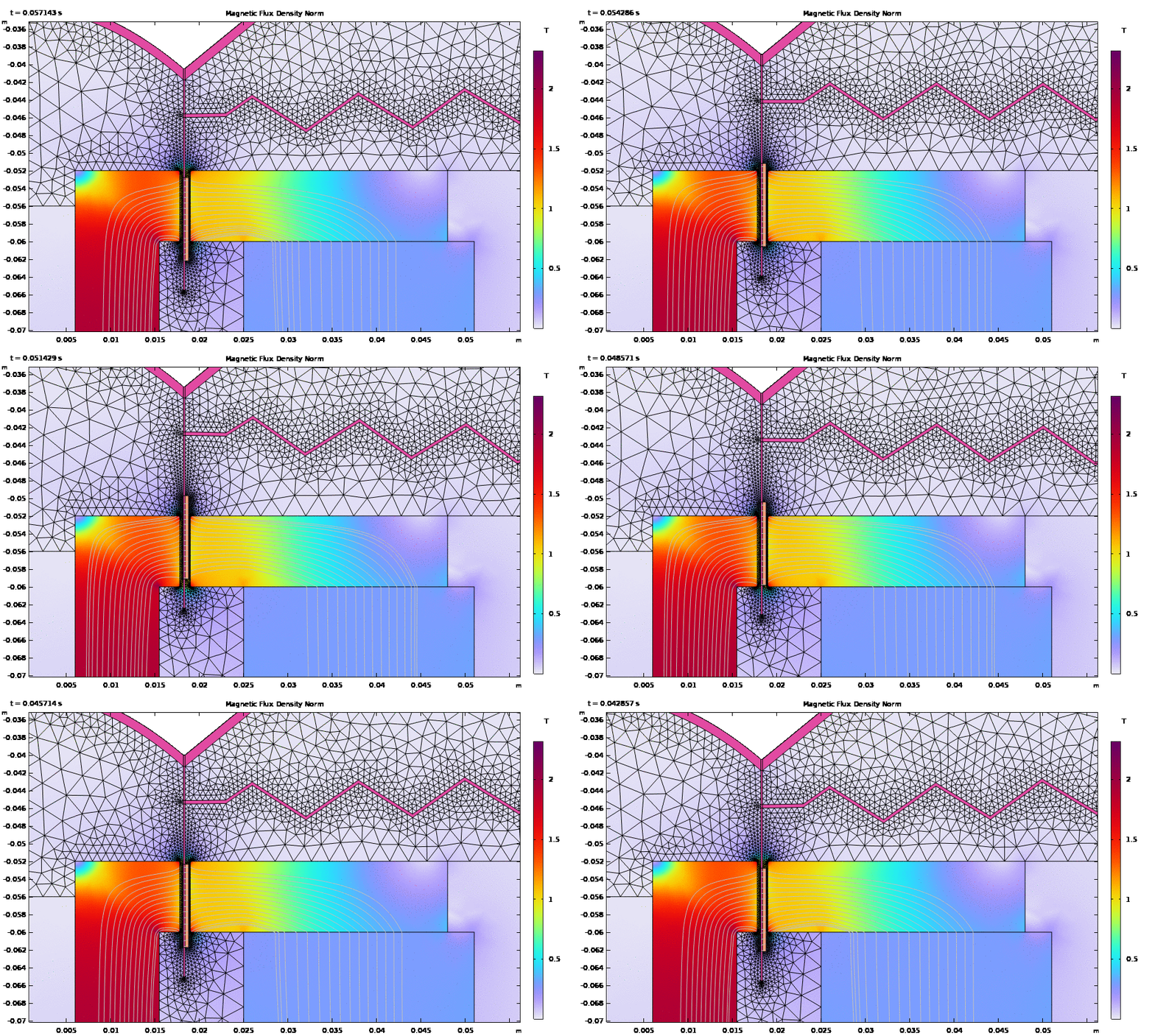
Magnetic field in and around the voice coil gap and the motion of the moving parts and mesh deformation during the time period of 3T0 to 4T0.
The plot below depicts the relative position of the voice coil, calculated as the vertical displacement from its original position averaged over the coil domain. The coil reaches its lowest position at 0.0437 s (green marker) and its highest position at 0.0509 s (red marker). At 0.048 s (cyan marker) and 0.055 s (magenta marker), the coil is on its way up and down, respectively.
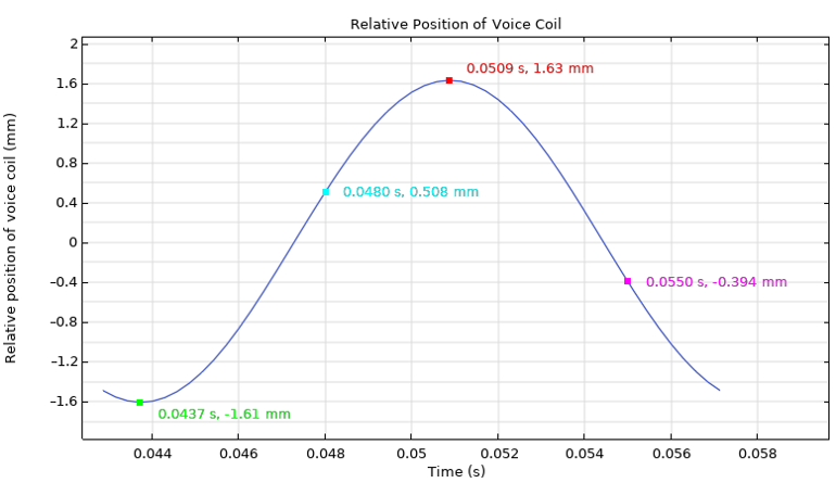
Relative position of the voice coil.
The distribution of the acoustic pressure around the speaker driver at these four time steps — 0.0437 s (top left), 0.048 s (top right), 0.0509 s (bottom left), and 0.055 s (bottom right) — are shown in the figure below. You can also see how the PML attenuates the acoustic waves generated by the motion of the speaker cone.
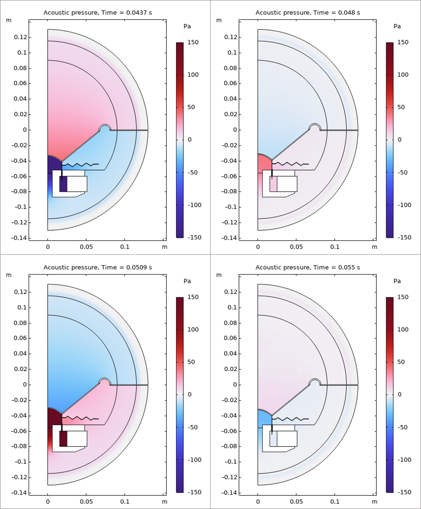 Four images showing the acoustic pressure at different time steps.
Acoustic pressure at 4 different time steps.
The acoustic particle velocity in the magnetic air gap at the lowest and highest coil positions is shown in the figure below. The velocity approaches zero at the walls due to the applied No Slip condition, resolving the viscous boundary layers and the associated damping in the narrow gap. Accurately capturing this damping is particularly important near resonance.
 The Acoustic particle velocity in the magetic air gap is visualized at time 0.0437s (left) and at time 0.0509 (right).
Acoustic particle velocity in the magnetic air gap at the lowest (left) and highest (right) positions of the voice coil.
Total Harmonic Distortion (THD) Calculation
An important output of interest of this analysis is the total harmonic distortion of the acoustic signals produced by the system. Distortion analyses, including the total harmonic distortion (THD) and intermodulation distortion (IMD), are commonly used to judge the quality of a speaker driver. These nonlinear effects produce overtones and additional nonharmonic frequency components, the extent of which can be quantified and calculated using the approaches discussed in our blog post "How to Perform a Nonlinear Distortion Analysis of a Loudspeaker Driver ". To calculate THD, we first need to choose a point of interest as a listening point, and obtain the frequency spectrum of the steady-state acoustic pressure at this listening point. The value of THD is then calculated as

where HN is the harmonic response of the Nth harmonic and H1 is the fundamental response.
Here, we choose the listening point at r = 0 and z = 0.115 m, the highest point in the physical domain lying on the acoustic axis. It is assumed that the speaker reaches the steady state by time t=3T0, and therefore the pressure signal as a function of time from t=3T0 to t=4T0 at this specific listening point is the steady-state solution that can be used for THD calculation, as seen in the plot below. You can see that the profile slightly differs from a perfect sinusoidal. This means that the output signal also contains frequency components other than f0.
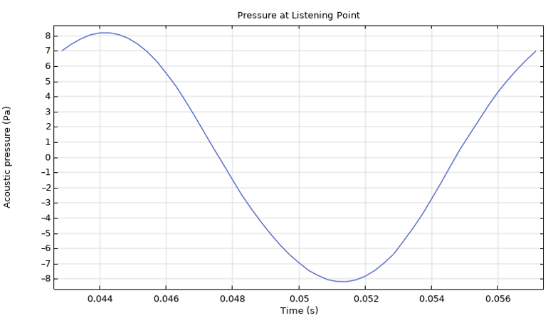
Acoustic pressure at the listening point.
Note that the accuracy of the FFT computation becomes higher for longer time intervals. Therefore, in order to obtain more accurate frequency spectrum of this one cycle signal, we perform a periodic extension of the data over time. This is done by the following steps:
1) Use a Point Evaluation feature to evaluate the pressure at the listening point from 3T0 to 4T0 with a time step of T0/50. This creates a table that stores the acoustic pressure as a function of time. See the Pressure at Point node under Results > Derived Values in the attached model file.
 The Pressure at Point node selected in the Model Builder and the Settings window with the Data, Selection, and Expressions sections expanded. In the Graphics window the pressure point is highlighted in blue. The pressure at listening points and the corresponding time is shown in the Pressure at Point table.
Point Evaluation is used to create a table storing acoustic pressure at the listening point.
2) Define an Interpolation function using the Result table as the data source and the table created from Step 1. The signal is interpolated by a cubic spline. See the Interpolation 1 (p_point) node under Global Definitions.
 The Model Builder with the Interpolation node selected and the Settings window with the Definition, Data Column Settings, and the Interpolation and Extrapolation sections expanded. In the Graphics window the function plot of the interpolated signal is plotted.
The interpolation function uses the result table as source data.
3) Define an Analytic function using the interpolation function specified in Step 2 and make it periodic through the Periodic Extension. See the Analytic 1 (p_periodic) node under Global Definitions. The extended pressure signal is seen below.
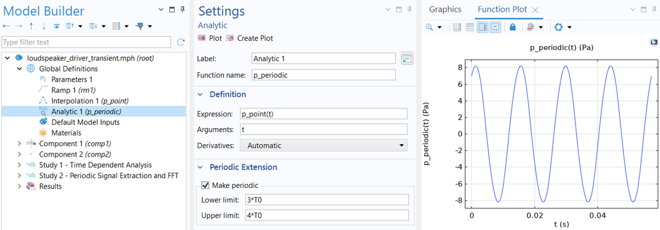 The Model Builder with the Analytics node selected and the Settings window showing the Definition and Periodic Extension section. In the Graphics window, the Function Plot of the expression p_point(t) is plotted.
A periodic extension of the pressure signal at the listening point.
The frequency spectrum analysis of the extended signal is then taken care of by the Global ODEs and DAEs interface defined in Component 2 and the second study, as seen in the images below. The study here consists of a Time Dependent and Time to Frequency FFT step. The first study step solves a global equation that passes the values of the periodically extended signal to a dependent variable named P; the second study computes the FFT of P. The first step is necessary because a Time to Frequency FFT study performs a forward FFT on only a dependent variable that an interface solves for. Here, we choose to extend the signal to 10 acoustic cycles for more accurate FFT computation.
 A close-up of Global Equations selected in the Model Builder and the corresponding Settings window with the Global Equations table for variable P.
The periodic extension of the pressure signal is passed onto a dependent variable, P, solved by a Global ODEs and DAEs interface.
 The Model Builder with the Time Dependent study selected and the Settings window showing the Study Settings and Physics and Variables Selection table.
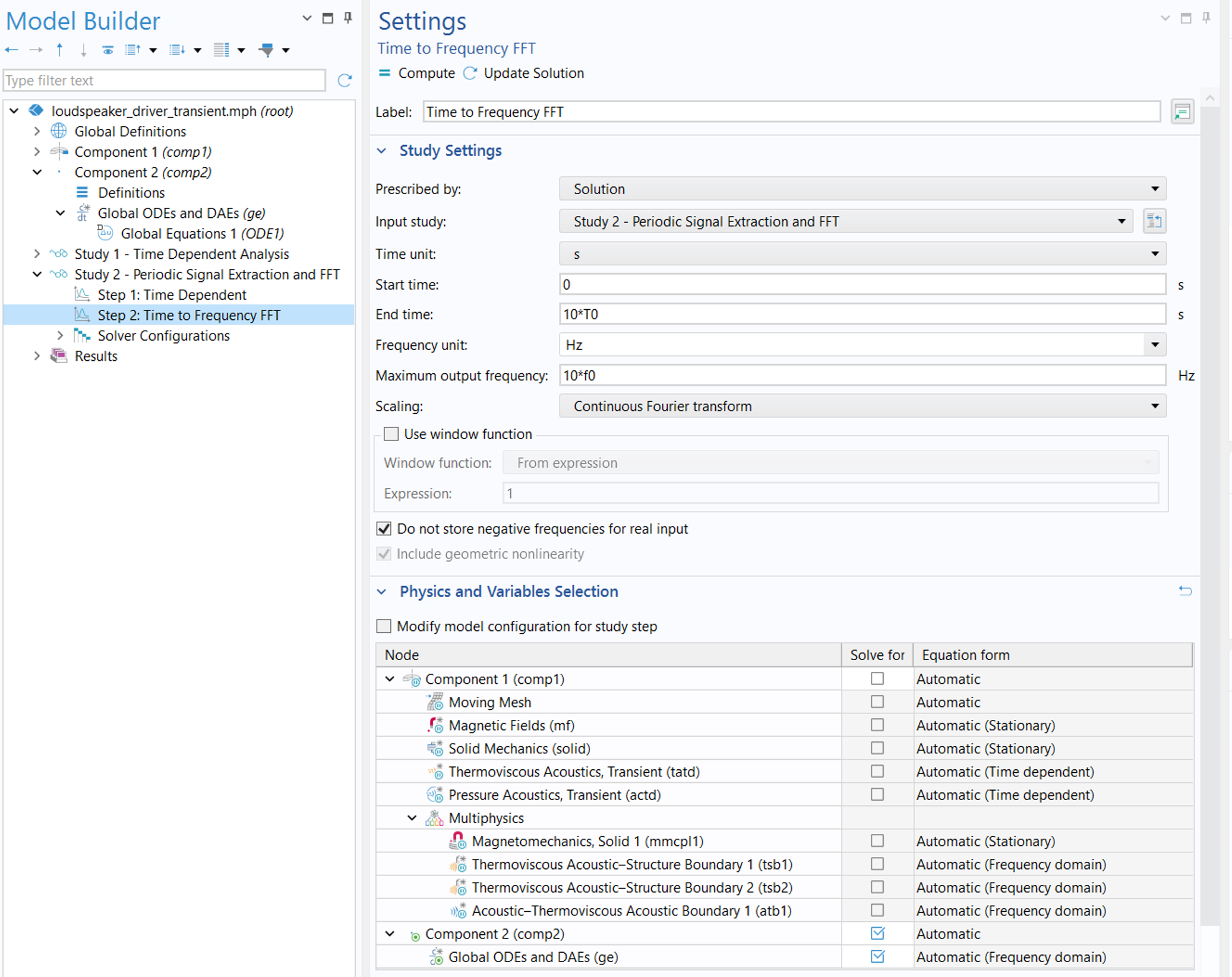 The Model Builder with the Time to Frequency FFT study selected and the Settings window showing the Study Settings and the Physics and Variables Selection table.
Study steps used for the frequency spectrum analysis of the extended signal.
The figure below shows the frequency spectrum of the acoustic signal obtained from the FFT study as the value of SPL over frequency. The highest peaks appear at frequencies that are multiples of f0 (red dots), and it is notable that the SPL for the odd-order harmonics is higher than that for the even-order harmonics, which means the symmetrical system nonlinearities dominate the asymmetrical ones.
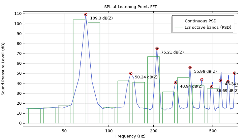 A graph showing the 1/3 octave bands (PSD) as green bar graphs and the continuous PSD as a blue line, with both lines peaking after 50 Hz.
The frequency spectrum of the acoustic signal (represented as SPL over frequency) at the listening point.
The THD value is computed in Derived Values > THD Evaluation using Global Evaluation with the following expression:
sqrt(sum(with(11 + 10*k, abs(comp2.P)^2), k, 1, 9))/with(11, abs(comp2.P))
 The Model Builder with Global Evaluation selected and the corresponding Settings window showing the dataset data and the calculated expression.
THD calculation using Global Evaluation.
The expression uses the with operator to access the solution of a specific frequency component and the sum operator to compute the sum of the expressions for all index values. More specifically, with(11, abs(comp2.P)) provides the acoustic pressure amplitude for the fundamental frequency (the 11th output frequency is 70 Hz), and sum(with(11 + 10*k, abs(comp2.P)^2), k, 1, 9), where k is the summation index, calculates the sum of the squared pressure amplitude of the first 9 harmonics. If you take a look at the output frequencies from the FFT study, you will see the index corresponding to the fundamental frequency and its harmonics. Such a calculation of including 9 harmonics yields a THD close to 2%.
Further Learning
This tutorial model and detailed documentation with step-by-step analysis instructions are also available for download in the Application Gallery: Loudspeaker Driver — Transient Analysis.
Submit feedback about this page or contact support here.