The Application Gallery features COMSOL Multiphysics® tutorial and demo app files pertinent to the electrical, structural, acoustics, fluid, heat, and chemical disciplines. You can use these examples as a starting point for your own simulation work by downloading the tutorial model or demo app file and its accompanying instructions.
Search for tutorials and apps relevant to your area of expertise via the Quick Search feature. Note that many of the examples featured here can also be accessed via the Application Libraries that are built into the COMSOL Multiphysics® software and available from the File menu.
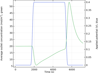
This example models the desalination of water by capacitive deionization in a "flow-between" cell (fbCDI). The model geometry is in 2D. Steady Brinkman flow, a tertiary current distribution, and the improved modified Donnan description of the deionization process is assumed. Read More

This model shows how to control the position of the base of an inverted pendulum to keep it vertical. The control is performed using a PID controller in Simulink®. The position of the base is constrained within specified limits, and an external force is applied at the base to keep it ... Read More
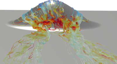
The present example simulates the turbulent flow over a 3D hill geometry using the Large Eddy Simulation (LES) interface with synthetic turbulence at the inlet boundary. Read More

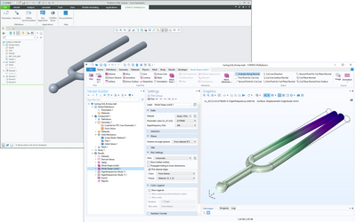
This model computes the fundamental eigenfrequency and eigenmode for a tuning fork that is synchronized from SOLIDWORKS® via the LiveLink™ interface. The length of the fork is then optimized so that the tuning fork sounds the note A, 440 Hz. Read More
This model computes the fundamental eigenfrequency and eigenmode for a tuning fork that is synchronized from Solid Edge® via the LiveLink™ interface. The length of the fork is then optimized so that the tuning fork sounds the note A, 440 Hz. Read More
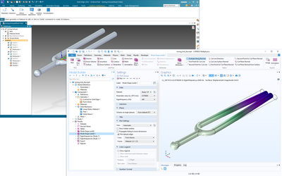
This model computes the fundamental eigenfrequency and eigenmode for a tuning fork that is synchronized from PTC Creo Parametric™ via the LiveLink™ interface. The length of the fork is then optimized so that the tuning fork sounds the note A, 440 Hz. Read More
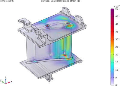
This example shows how to compute deformations caused by secondary creep in a turbine stator blade. The creep rate is highly influenced by temperature, and the deformation and stress relaxation is thus controlled by the temperature field. Read More
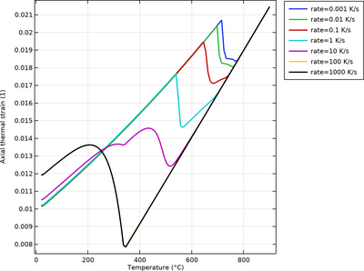
In this example, phase transformation data and phase material properties are imported from JMatPro, and used to compute CCT curves. Dilatometry curves (axial thermal strain) are computed across a range of cooling rates. Read More

This tutorial model shows the setup of a 2D axisymmetric stress analysis, through contact, of a 3D threaded pipe fitting. The example involves synchronizing the 3D Solid Edge® geometry and selections, which specify the faces in contact, with the 2D geometry in COMSOL ... Read More
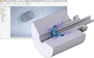
This tutorial model shows the setup of a 2D axisymmetric stress analysis, through contact, of a 3D threaded pipe fitting. The example involves synchronizing the 3D Inventor® geometry and selections, which specify the faces in contact, with the 2D geometry in COMSOL Multiphysics ... Read More