The Application Gallery features COMSOL Multiphysics® tutorial and demo app files pertinent to the electrical, structural, acoustics, fluid, heat, and chemical disciplines. You can use these examples as a starting point for your own simulation work by downloading the tutorial model or demo app file and its accompanying instructions.
Search for tutorials and apps relevant to your area of expertise via the Quick Search feature. Note that many of the examples featured here can also be accessed via the Application Libraries that are built into the COMSOL Multiphysics® software and available from the File menu.
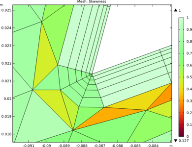
Tutorials in this series deal with creating and manipulation of boundary layer meshes. In these tutorials you will learn how to set up a boundary layer mesh and modify the settings for an automatically created boundary layer mesh. For physics-controlled meshing a boundary layer mesh is ... Read More
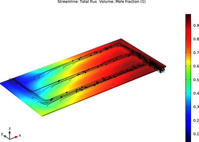
This example models a solid oxide electrolyzer cell wherein water vapor is reduced to form hydrogen gas on the cathode, and oxygen gas is evolved on the anode. The current distribution in the cell is coupled to the cathode mass transfer of hydrogen and water and momentum transport. Two ... Read More

Different types of elements can be used for modeling a rotor, depending on the level of complexity and the type of the system being modeled. The modeling steps and representation of the results will vary with the type of idealization. In this tutorial model, an eigenfrequency analysis is ... Read More

This is a template MPH-file containing the physics interfaces and the parameterized geometry for the model Electrical Heating in a Busbar. Read More

This is a full vibro-electroacoustic simulation of a balanced armature transducer (BAT or also known as a receiver in some industries) which is a high-performance miniature loudspeaker often used in hearing aids and other in-ear audio products such as earbuds. The model is set up and ... Read More

Headphones are closely coupled to the ear, and so it is not possible to measure their sensitivity in a classical acoustic free-field setup used for loudspeakers. The measurement requires the use of artificial heads and ears to accurately represent the usage conditions. This model shows ... Read More
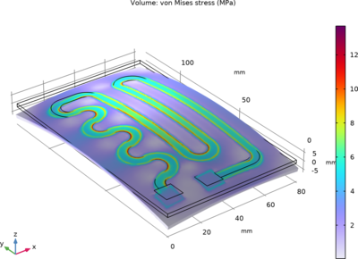
Small heating circuits find use in many applications. For example, in manufacturing processes, they heat up reactive fluids. The device in this tutorial example consists of an electrically resistive layer deposited on a glass plate. The layer results in Joule heating when a voltage is ... Read More
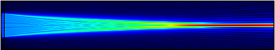
Optical lenses of millimeter size cannot easily be analyzed with the Electromagnetic Waves, Frequency Domain interface on standard workstations due to the large number of finite element mesh elements required. This model explains how the Electromagnetic Waves, Beam Envelopes interface ... Read More

This alternative version of the Tubular Reactor app demonstrates how computational speed can be significantly increased by using a surrogate model instead of a full finite element model. A surrogate model is a simplified, computationally efficient approximation of a more complex and ... Read More
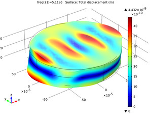
AT cut quartz crystals are widely employed in a range of applications, from oscillators to microbalances. One of the important properties of the AT cut is that the resonant frequency of the crystal is temperature independent to first order. This is desirable in both mass sensing and ... Read More