Applying Translations, Scaling, Reflection, and Rotation via the Deformed Geometry and Moving Mesh Interfaces
The Deformed Geometry and Moving Mesh interfaces are useful for modeling situations where a domain is deforming, as well as when it is moving in a completely prescribed way, either as a function of time or as a function of a model parameter in a parametric sweep or auxiliary sweep. Using these interfaces usually avoids any remeshing of the geometry or solving of additional equations.
The Moving Mesh and Deformed Geometry Interfaces
In most cases, the Moving Mesh interface is the appropriate interface to use, since in this interface, the material, and solution, moves with the spatial deformation. The Deformed Geometry interface, on the other hand, implies that material is being added and removed from a domain as it translates through space, and is appropriate for models involving the Solid Mechanics interfaces, which themselves compute a deformation of the solid material as defined on the Material frame. It is not possible to solve for both Solid Mechanics and Moving Mesh within the same domain. Another way to keep track of this is in terms of these three frames:
- Geometry frame coordinates, default
 , are fixed in the CAD geometry in 3D.
 - Material frame coordinates, default
 , are fixed in the material in solid domains. A difference between Material and Geometry frame coordinates may be induced by Deformed Geometry or Shape Optimization features in the model. The difference represents a different configuration of the material, i.e., effectively a different shape of solid objects.
 - Spatial frame coordinates, default
 , are fixed in space. A difference between the Spatial and Material frame coordinates may be induced by Moving Mesh features or structural mechanics interfaces, which control the Spatial frame. The difference represents a displacement of the material.
To verify which frame is being used for making plots, use the Frame setting within a Dataset feature, as shown in the screenshot below. Each plot group can also plot the edges of the dataset, in a selected frame, as shown below.
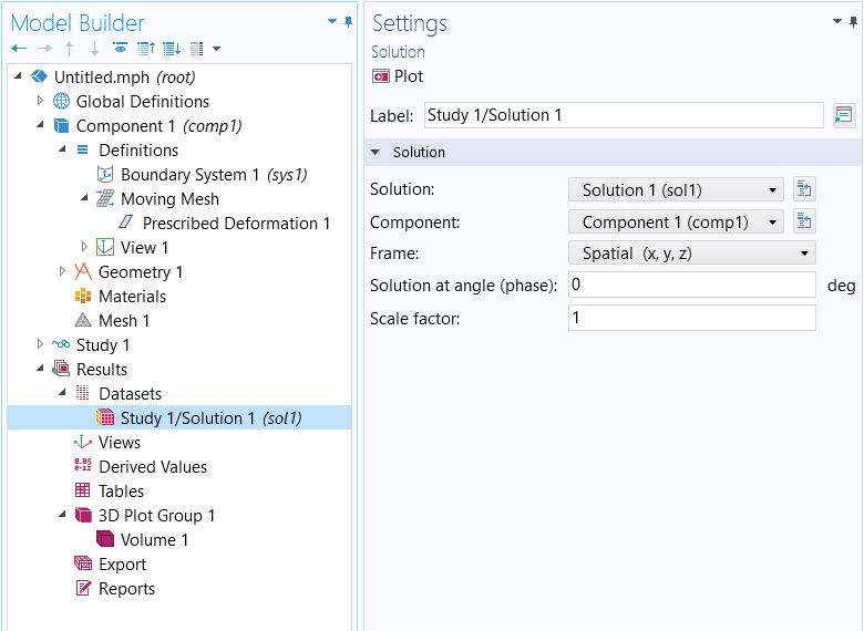
Screenshot showing how to select the frame used to plot results.
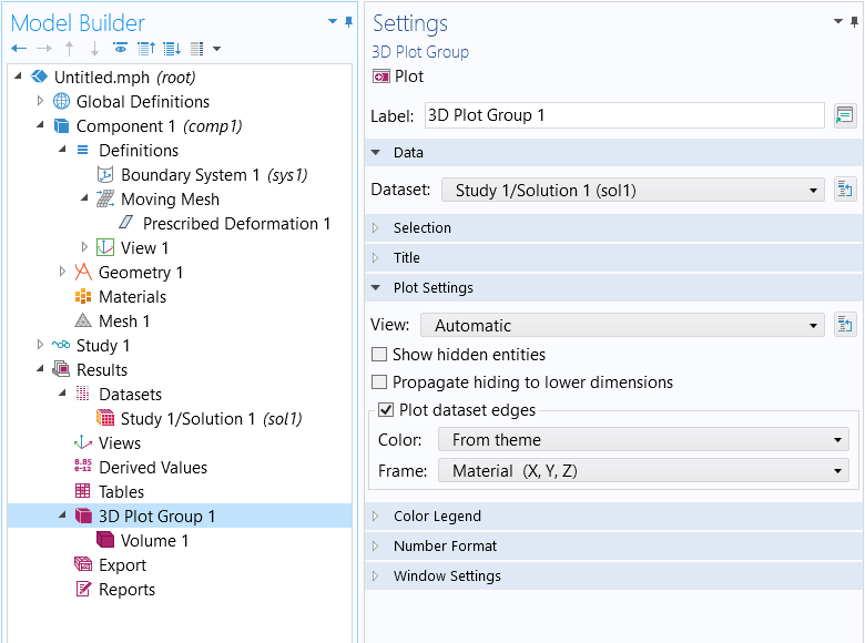
Within each plot group, it is also possible to plot the dataset edges, using different frames.
Modeling Translations
To model the translation of a domain, such as for the movement of a part in space, define the expression of a translation curve in space:  . Use these expressions within a Moving Mesh > Prescribed Deformation feature such that every point within the domain is offset from its original location by the same amount.
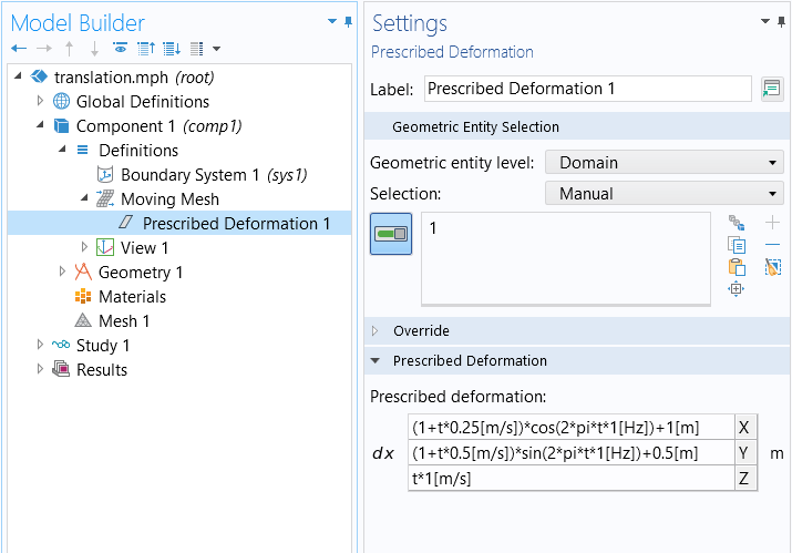
Using the Prescribed Deformation feature to implement translation.
For example, to move a domain along a helical spiral path centered along a line parallel to the Z-axis and offset from its original position, use these expressions for the prescribed deformation:
dx = (1[m]+t*0.25[m/s])*cos(2*pi*t*1[Hz])+1[m]
dy = (1[m]+t*0.5[m/s])*sin(2*pi*t*1[Hz])+0.5[m]
dz = t*1[m/s]
This translation example is shown in the above screenshot and implemented in the exercise file.
Modeling Scaling & Reflection
To model a domain that is expanding or contracting about the global Cartesian coordinate system, it is necessary to define a scale factor matrix and a point to scale about. The scale factor matrix,  , is a diagonal matrix with entries corresponding to scaling the Cartesian directions. For example:

will leave the x-dimensions unchanged, scale the y-dimension up by two, and reduce the z-dimension by half.
It is also necessary to define the point about which the domain is scaled,  , and this defines the deformation field of the domain:

where  is the identity matrix.
So, for example, to scale a part about the point 1,2,3 by the above scale factor matrix, prescribe a deformation of:
dx = (1-1)*(X-1[m])
dy = (2-1)*(Y-2[m])
dz = (0.5-1)*(Z-3[m])
It is also possible to make the terms functions of time or other model parameters. An example is implemented in the exercise file.
Modeling Rotations, Scaling, and Translations
Modeling of generalized rotation can become complex. Two cases are addressed here: rotation about a Cartesian axis, as well as a more general case of 3D rotation.
For rotations about one of the global Cartesian axes, it is sufficient to define a single rotation matrix, and the coordinate of the center of rotation. For example, consider rotating a part through an angle theta about a line parallel to the Z-axis and passing through the point  . The rotation matrix about any line parallel to the Z-axis is:

And, to rotate about the point , use the deformation:

This is equivalent to using the Rotating Domain feature. An example is included in the exercise file.
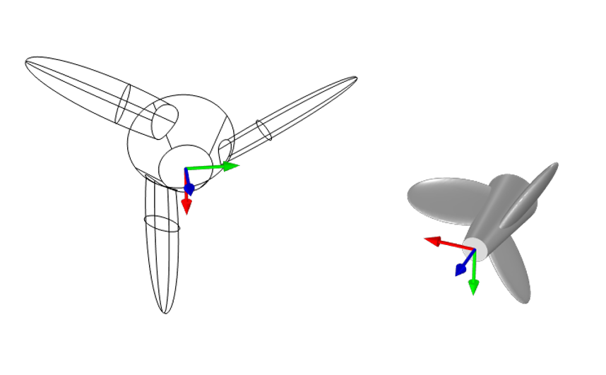
For the more general case of a part rotated and moved arbitrarily in space, two coordinate systems need to be conceptually defined,  and
and  , at points
  and
and  , as shown in the image below. Consider the first, , as algined with the part. The objective is to rotate and move the part to align the part coordinate system with .
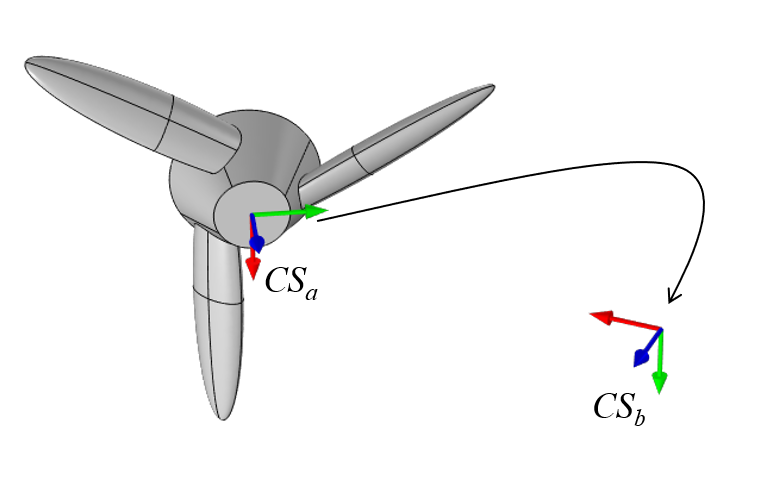
A part with a coordinate system that will be rotated and moved to align with a second coordinate system. The first, second, and third axes of these systems are shown in red, green, and blue, respectively.
Both coordinate systems are defined in terms of two orthonormal vectors,  &
&  , with the third vector defined by the cross-product:
  . These vectors define a transformation matrix:

This transformation matrix will rotate the part from one coordinate system to another. The above matrix is equivalent to applying a rotation that rotates the part from into the global Cartesian CS. This rotation should be done about , and then, to rotate from the global Cartesian to and move to point , use the following expression for deformation:

It is also possible to include a scaling. To do so in the coordinate system, use a combined scaling, rotation, and translation via an expression of:

An example of this is in the exercise file.
Translation and anisotropic scaling applied, as well as rotation, in terms of two coordinate systems. The original undeformed part is shown in wireframe.
Submit feedback about this page or contact support here.