Learning Center

Finite Element Frequency-Domain Analysis in 2D

---

In this part of the course, we will learn how to set up a model for a frequency-domain analysis in the 2D axisymmetric space dimension using the Model Wizard in COMSOL Multiphysics^®. The rotationally symmetric driver is placed in an infinite baffle with free space in front of and on the back of the speaker.

The Model Wizard

Start by setting up a new model. To do this, select File > New. In the Model Wizard, select 2D Axisymmetric as the space dimension, as shown in the figure below.

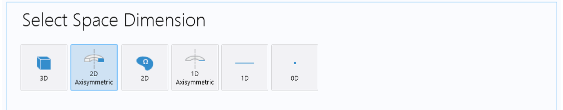Selecting 2D Axisymmetric for the space dimension in the Model Wizard.

Next, from the Select Physics page of the Model Wizard, select the Magnetic Fields interface, which is under the AC/DC > Electromagnetic Fields branch, and then click Add.

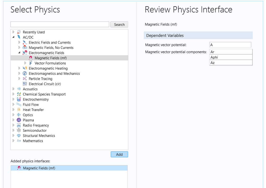The Magnetic Fields interface is under the AC/DC > Electromagnetic Fields branch in the Select Physics page of the Model Wizard.

Next, select the Acoustic-Solid Interaction, Frequency Domain interface from the Acoustics > Acoustic-Structure Interaction branch, as shown below. This adds a Pressure Acoustics, Frequency Domain interface for modeling pressure waves in fluids; a Solid Mechanics interface for modeling elastic waves in solids; and a Multiphysics > Acoustic-Structure Boundary feature that couples the two interfaces. Note that this can also be achieved by first adding each physics one at a time, and then adding the Acoustic-Structure Boundary coupling in the Model Builder.

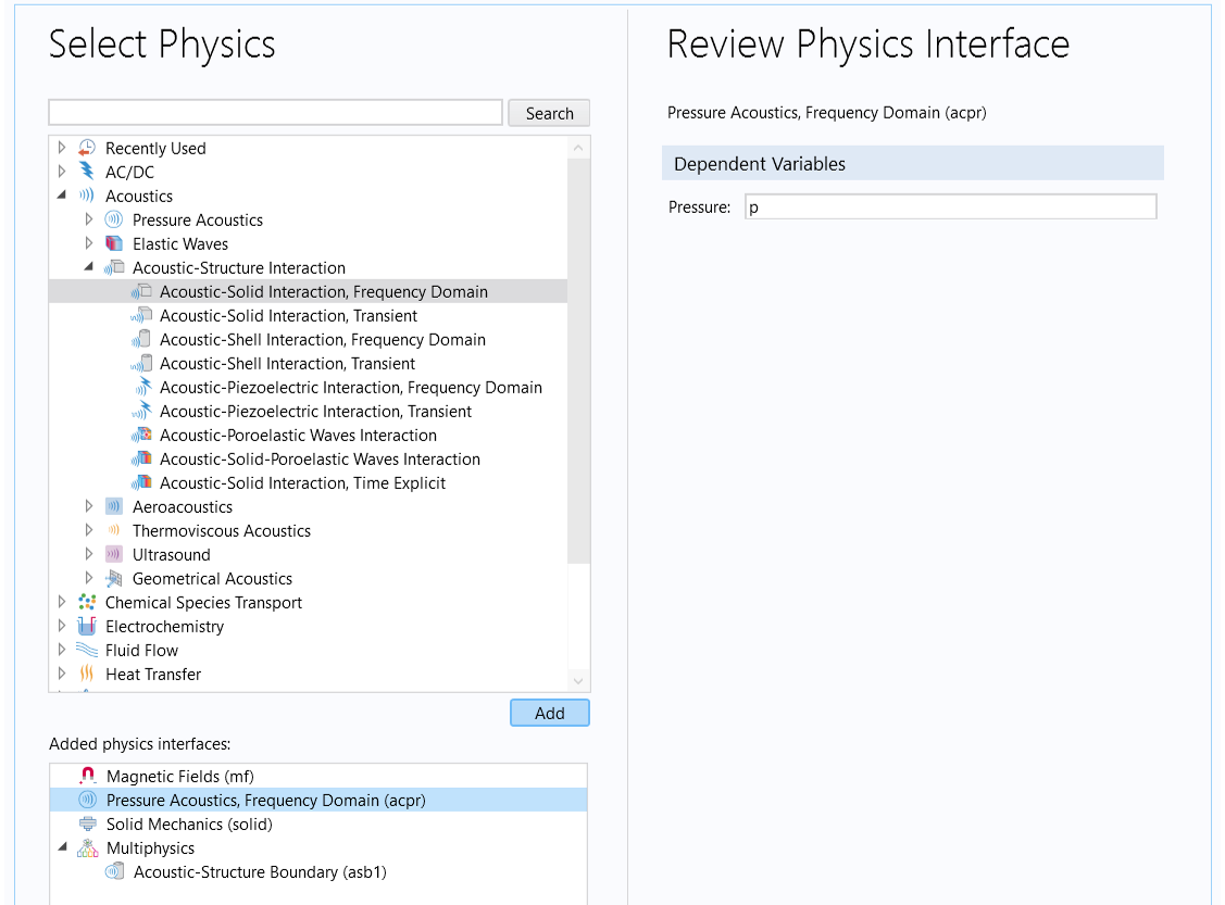The Acoustic-Solid Interaction, Frequency Domain multiphysics interface is under the Acoustics > Acoustic-Structure Interaction branch of the Select Physics page of the Model Wizard.

The last step in the Model Wizard is to select the study type. As explained in Part 1, you have two options to create the two-step study for a Frequency Domain, Perturbation analysis:

1. First, select the Stationary study type from Preset Studies for Some Physics Interfaces at the Select Study step of the Model Wizard. The second study step, Frequency Domain Perturbation, will be manually added later.
2. Select the Small-Signal Analysis, Frequency Domain study from the Magnetic Fields interface, as shown in the image below. This study consists of the two required study steps: a Stationary study step for computing the biased solution and a Frequency Domain, Perturbation study step for computing the frequency response about the biased solution.

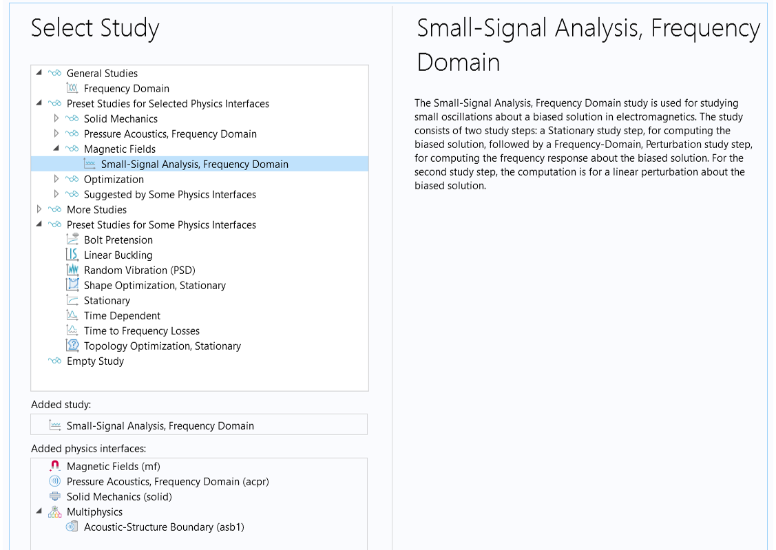The Small-Signal Analysis, Frequency Domain study consists of the two required study steps for a full electrovibroacoustic analysis.

Let's use the second option here and click Done to enter the Model Builder workspace.

Parameters

We need to define a few parameters to be used in the model setup. These include the number of turns in the coil, ; the peak driving voltage, ; the frequency at which the loss factor is given (this is for use in the Rayleigh damping model definitions in some of the structural parts), ; the angular frequency at which the loss factor is given, ; the maximal study frequency, ; the speed of sound in air, ; and the minimum wavelength, .

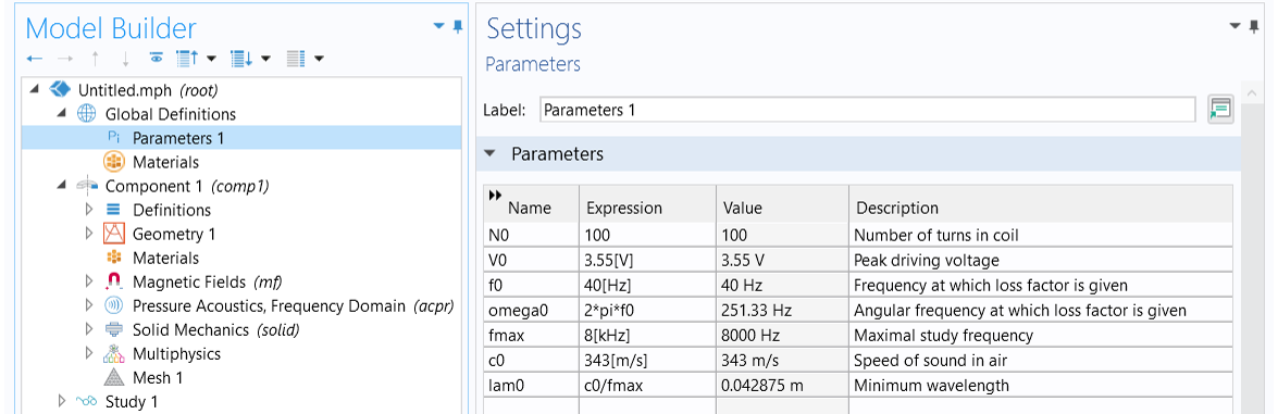The parameters used in the model.

Geometry

In this exercise, we import the geometry sequence created in the model file, dynamic_speaker_driver.mph, attached in the sidebar. Therefore, you need to first download the model file and save it to your local computer. Then perform the following steps:

1. Right-click the Geometry 1 node and select Insert Sequence From.
2. Browse to the folder where the file named dynamic_speaker_driver.mph is saved and click Open.
3. Click Build All.

The geometry sequence and named domain selections are added to the model. The selections for the magnet, the pole piece and top plate, the coil, the former, the spider, the cone, the surround, and the air field represented by a half-circle can be used through the modeling workflow. An image of the imported 2D axisymmetric geometry is shown below. (For simplicity, the speaker basket has been omitted from this model.) Refer to named selections to learn more.

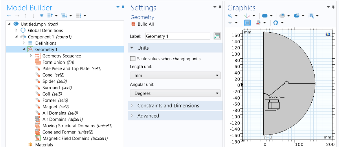The geometry is created by inserting the geometry sequence from the dynamic_speaker_driver.mph file.

Domain Selections for the Physics Interfaces

By default, all domains in the geometry are included in every physics interface added to the model. Making the correct domain selections is an important step in the model setup.

For the Magnetic Fields interface, choose Magnetic Field Domains from the drop-down Selection list in the Domain Selection section. As shown in the image below, these are the domains underneath the diaphragm that includes all the electromagnetic components, i.e., the magnet, the soft iron pole piece and top plate, the coil, and the former, as well as the spider and the air domain below the cone.

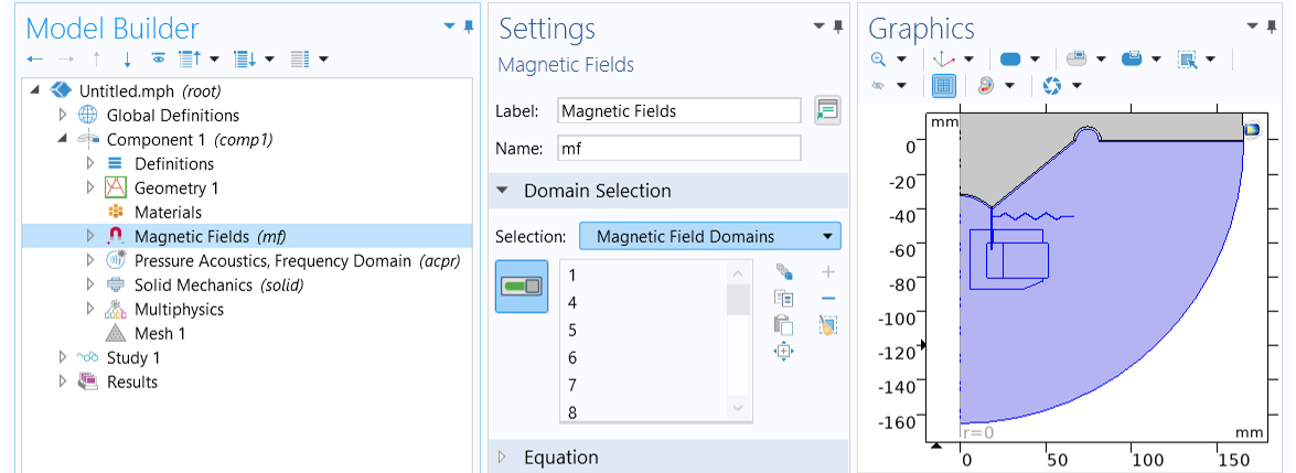Select Magnetic Field Domains in the Domain Selection section of the Settings window for the Magnetic Fields interface.

For the Pressure Acoustics, Frequency Domain interface, choose Air Domains from the drop-down Selection list in the Domain Selection section. It includes the air domains above and beneath the cone.

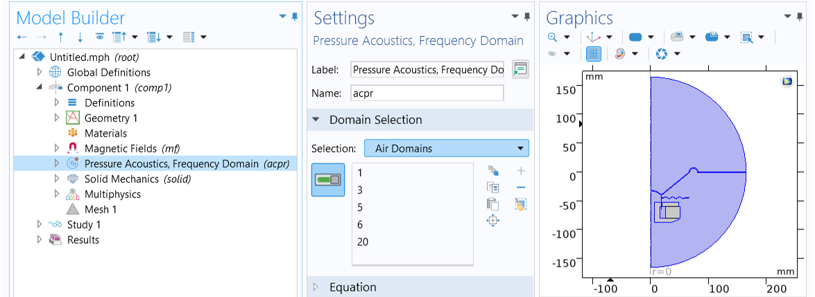Select Air Domains in the Domain Selection section of the Settings window for the Pressure Acoustics, Frequency Domain interface.

For the Solid Mechanics interface, choose the Moving Structural Domains option from the selection list in the Domain Selection section. It includes all of the moving parts, i.e., the coil, the former, the cone, the suspension, and the spider.

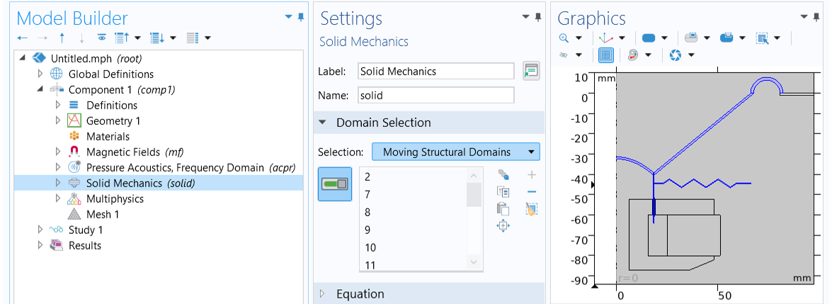Select Moving Structural Domains in the Domain Selection section in the Settings window for the Solid Mechanics interface.

Acoustic–Structure Boundary Coupling

Once you make the correct domain selections for the Pressure Acoustics, Frequency Domain and Solid Mechanics interfaces, the Acoustic-Structure Boundary coupling is automatically applied at the boundaries between the fluids and solids to ensure continuity.

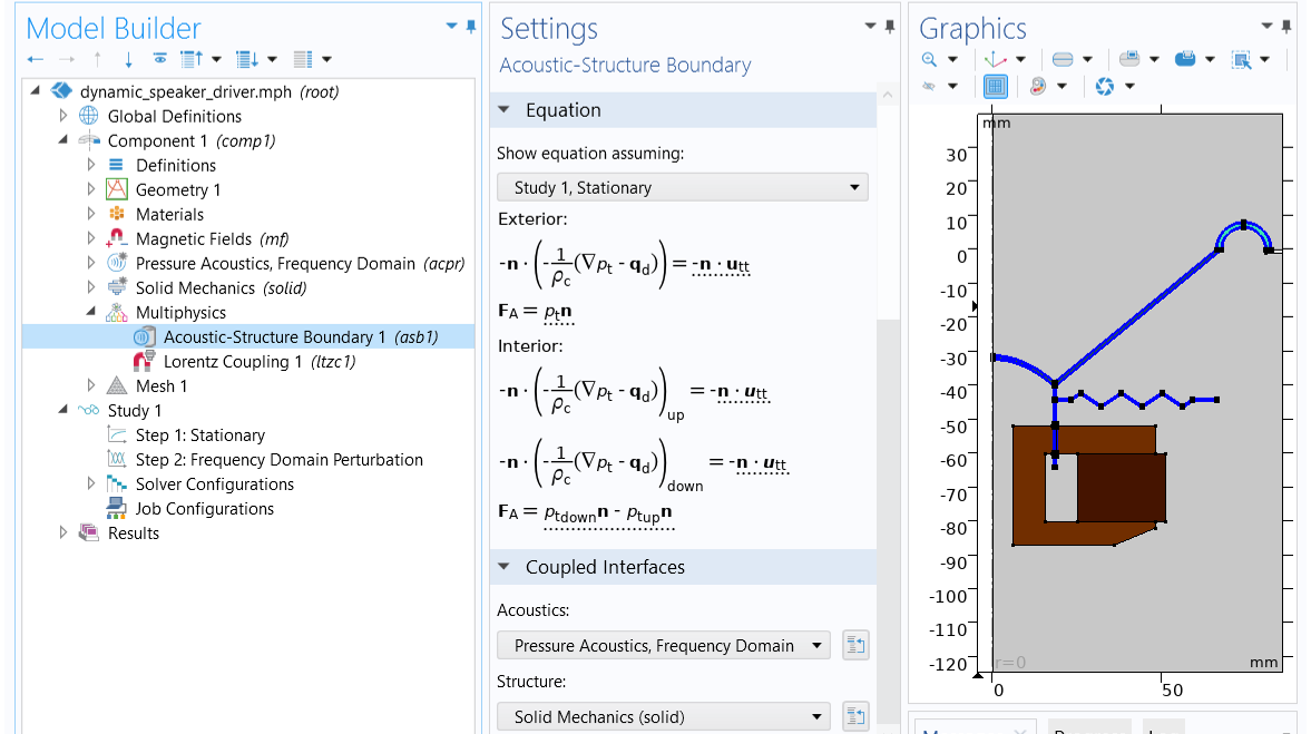The Model Builder with the Acoustic-Structure Boundary feature selected, the corresponding Settings window showing the equation settings and coupled interfaces, and the Graphics window showing the acoustic–structure boundaries where the coupling is applied. The Acoustic-Structure Boundary coupling is used to couple a pressure acoustics model with any structural component.

Magnetic Fields and Solid Mechanics Coupling

Next, couple the Magnetic Fields interface and Solid Mechanics interface. For previous versions (up through version 6.1), you can add a Lorentz Coupling feature, and for the current version, you can add a Magnetomechanics Coupling feature to the Multiphysics node to do this.

If you add a Lorentz Coupling feature choose Coil from the selection list in the Domain Selection section of the settings window as shown in the image below.

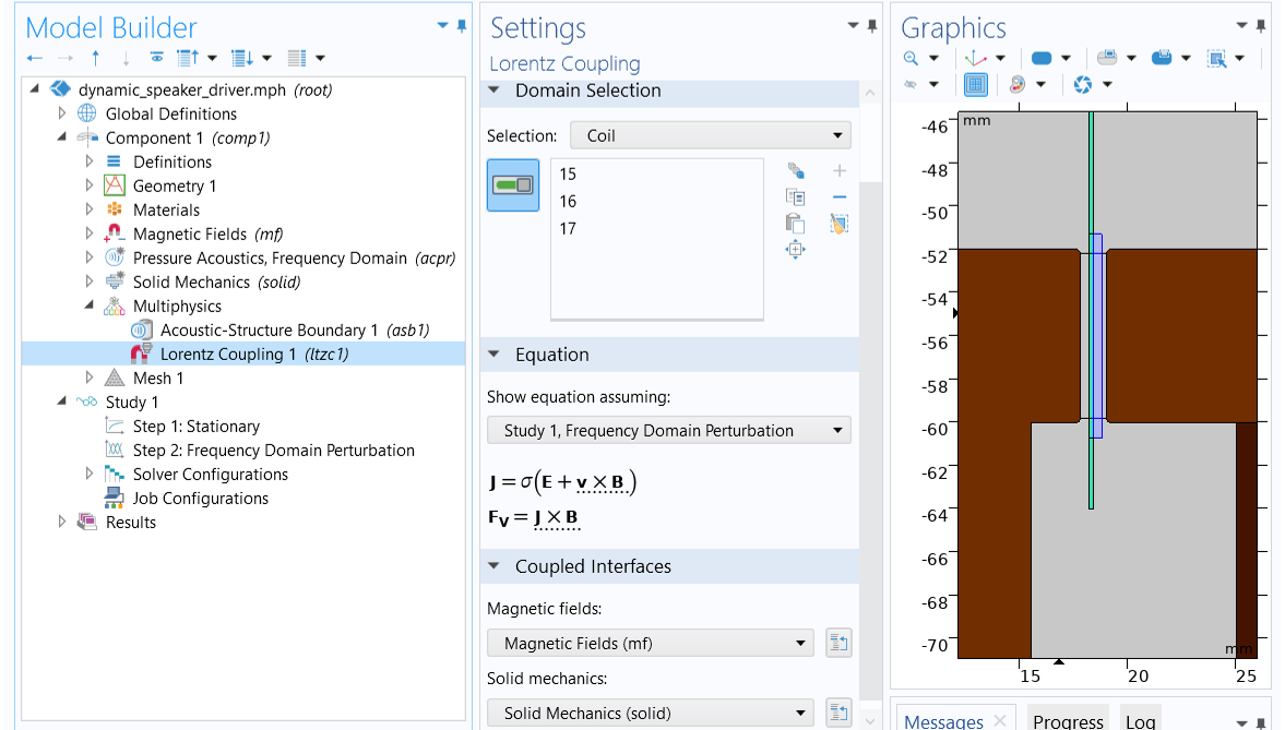The Model Builder with the Lorentz Coupling feature selected, the corresponding Settings window showing the equation settings and coupled interfaces, and the Graphics window showing the coil domains where the Lorentz Coupling is applied. The Lorentz Coupling is a multiphysics coupling feature between the Magnetic Fields interface and Solid Mechanics interface used through version 6.1.

If you add a Magnetomechanics Coupling feature, enable Only use Lorentz force and select Coil from the selection list in the Domain Selection section of the settings window to obtain an equivalent coupling. This method is shown in the image below.

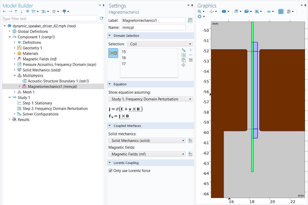The Model Builder with the Magnetomechanics Coupling feature selected, the corresponding Settings window showing the equation settings and coupled interfaces, and the Graphics window showing the coil domains where the Magnetomechanics Coupling is applied. The Magnetomechanics Coupling is a multiphysics coupling feature between the Magnetic Fields interface and Solid Mechanics interface used in the current version of COMSOL Multiphysics^®.

The Magnetic Fields Physics Setup

Magnetization Models for the Electromagnetic Components

The driver contains different electromagnetic components, and each has its specific constitutive relation that describes the macroscopic properties of the medium (relating the magnetic flux density, , and the magnetic field, ) and the applicable material properties. The default, Relative permeability, is a magnetization model that uses the relative permeability to define the constitutive relation . A different magnetization model needs to be used for the magnet and for the pole piece and top plate.

The Magnet

The magnet requires a Remanent Flux Density magnetization model that uses the constitutive relation , where and are the recoil permeability and the remanent flux density (the flux density when no magnetic field is present), respectively. To set this model up for the magnet:

1. Add an Ampère's Law domain feature to the Magnetic Fields interface.
2. In the Label edit box, change the label to Magnet.
3. Choose Magnet as the domain selection.
4. Choose Remanent Flux Density from the Magnetization model selection list in the Constitutive Relation B-H section.
5. Set the Remanent flux direction to be in the z direction, as shown in the image below.

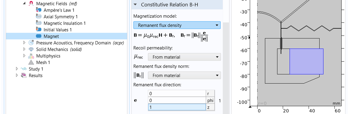Close-up views of the Model Builder, the Settings window with the Remanent flux density option selected for the magnet, and the Graphics window. The Remanent Flux Density magnetization model is used to model the constitutive relation for the magnet.

The Pole Piece and Top Plate

The soft iron in the pole piece and top plate is modeled as a nonlinear magnetic material, with the relationship between the B and H fields described by interpolation from measured data. This can be modeled using a B-H curve magnetization model, as shown in the image below.

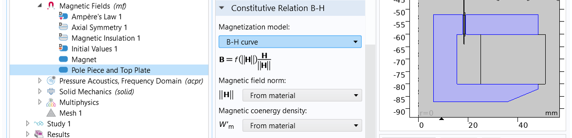Close-up views of the Model Builder, Settings window, and Graphics window, with the B-H curve option selected from the Magnetization model drop-down list. The B-H curve magnetization model is used to model the constitutive relation for the pole piece and top plate.

Coil

Although the voice coil consists of many turns of wire, it is, for simplicity, drawn and modeled as a homogenized domain using a Coil domain feature, as shown in the image below. The Homogenized multiturn option enables you to model a coil containing a large number of wires without the need to model each wire individually. In the Settings window for the Coil feature, perform the following steps:

1. Select Coil as the domain selection.
2. Choose the Homogenized multiturn option for the Conductor model in the Coil section.
3. Choose Voltage for Coil excitation.
4. Use linper(V0) to define Coil voltage. The linper() operator is used so that the coil excitation is applicable only in the Frequency Domain, Perturbation study step.
5. In the Homogenized Multiturn Conductor section, enter N0 for Number of turns and 3.5e-8[m^2] for Coil wire cross-section area. With N0 = 100 turns, the total cross-sectional area covered by the wires will be 3.5e-6 m². The area of the coil domain is 6e-6 m², making the fill factor (the ratio between the volume of the winding coil and the volume needed to house the winding coil) approximately 60%.

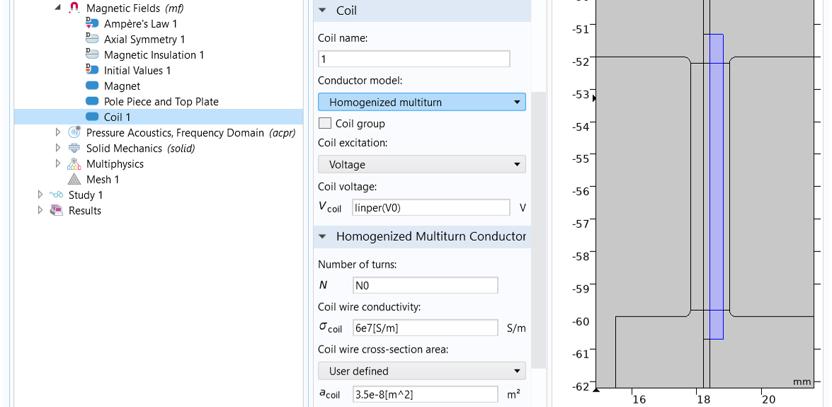A close-up of the Model Builder, the Coil settings window, and the Graphics window, with the Homogenized multiturn option selected in the Settings window. Settings for the homogenized multiturn coil.

The Pressure Acoustics, Frequency Domain Physics Setup

Open Boundaries

The air domains and the baffle should ideally extend to infinity. To avoid unphysical reflections where you truncate the open air field, use a Perfectly Matched Boundary feature, as seen in the image below. Add this node from the Radiation Conditions submenu.

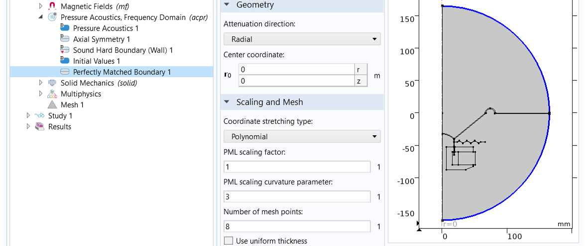The Perfectly Matched Boundary feature selected in the Model Builder, a close-up of the Geometry and Scaling and Mesh sections of the Settings window, and the model in the Graphics window. A Perfectly Matched Boundary feature is used at the open boundaries to avoid unphysical reflections.

The Perfectly Matched Boundary feature is effectively a perfectly matched layer (PML) that is applied to an open boundary without the need to define a domain (a layer in the geometry). The condition automatically applies the PML formulation using the extra dimension functionality of COMSOL Multiphysics^®. Here, we use the default settings as shown in the image above, i.e., the Attenuation direction is set as Radial, the Coordinate stretching type as Polynomial, the PML scaling factor to 1, the PML scaling curvature parameter to 3, and the Number of mesh points to 8.

Thermoviscous Damping in Narrow Gaps

In the narrow air gap between the top plate and the voice coil, and that between the pole piece and the former, damping occurs due to thermal and viscous boundary layer losses. These losses can be modeled in detail using a Thermoviscous Acoustics physics interface. However, since each gap here is well approximated by a slit of constant cross-section area, we can simply use the Narrow Region Acoustics feature available for the Pressure Acoustics, Frequency Domain interface. This equivalent fluid model has a low computational cost compared to a thermoviscous acoustic model. Since the two gaps have different widths, add two Narrow Region Acoustics nodes to the pressure acoustics model: one for the gap on the left (between the pole piece and the former), with the slit height set to 0.4[mm], and the other for the gap on the right (between the top plate and the voice coil), with the slit height set to 0.2[mm].

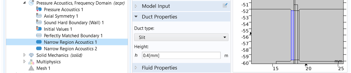
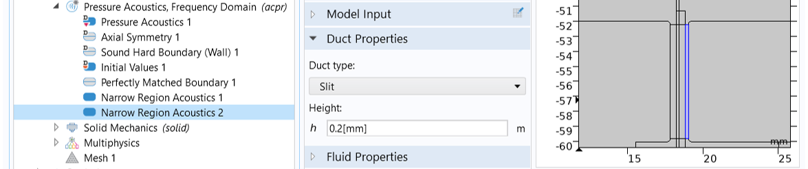The Narrow Region Acoustics feature is used to capture the thermal and viscous boundary layer losses in the narrow air gaps.

Exterior Field Calculation

The Perfectly Matched Boundary feature enables us to compute the acoustic pressure field inside a finite-sized air domain, however, we also often want the solution beyond the solved region. This can be achieved by using the Exterior Field Calculation to calculate and visualize the pressure field outside the computational domain at any distance including amplitude and phase. The exterior field boundary, the surface where the Exterior Field Calculation is applied, should be continuous and needs to enclose all sources and scatterers with the desired symmetry types. The solution outside the surface is calculated as a boundary integral, known as the Helmholtz-Kirchhoff integral, in terms of quantities evaluated on the surface.

In this example, the sound field above and below the infinite baffle is separated. To calculate the solution of the exterior field above the baffle, apply the feature to the exterior boundary of the air domain lying above the baffle and set the symmetric condition at , as shown in the image below.

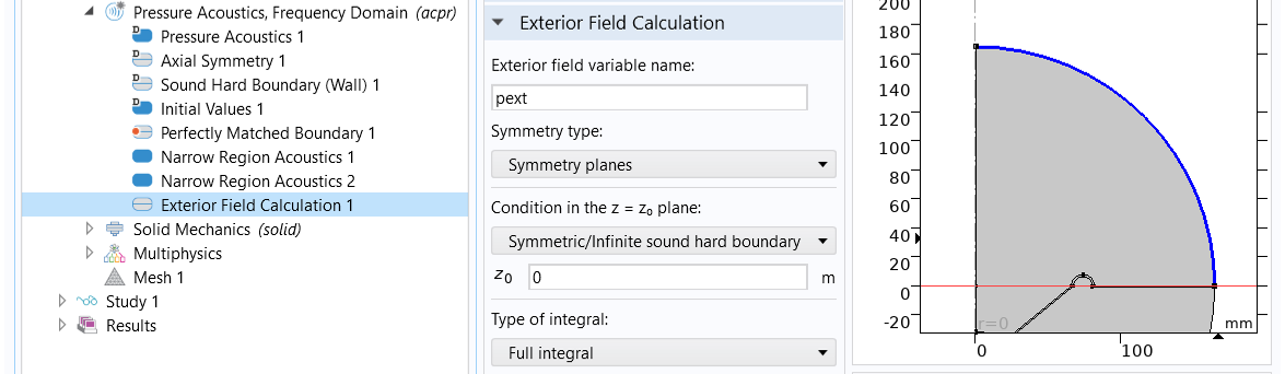The Exterior Field Calculation feature allows for the calculation and visualization of the pressure field outside the computational domain.

The Solid Mechanics Physics Setup

For the Solid Mechanics physics interface, make sure that appropriate material models are used for different moving parts and that constraints are applied to reflect how the vibration system is supported. In this study, the default isotropic Linear Elastic Material model is used for all structural components, with specific damping applied to each material domain.

Mechanical Damping to the Moving Components

Different damping models are available to include mechanical damping and losses, which are important factors for determining the dynamic response in vibrations analysis. For frequency-domain analysis there are four basic damping models available in the structural mechanics interfaces for explicit modeling of material damping: Rayleigh damping, Viscous damping, Loss factor, and Wave attenuation models, which are all based on introducing complex-valued quantities into the equation system. Here, we add isotropic loss factor damping to the cone and former and Rayleigh damping to the spider and surround. As seen in the image below, add a Damping subfeature to the Solid Mechanics interface > Linear Elastic Material 1 node, select Cone and Former in the Domain Selection section. In the Damping Settings section, choose Isotropic loss factor for Damping type.

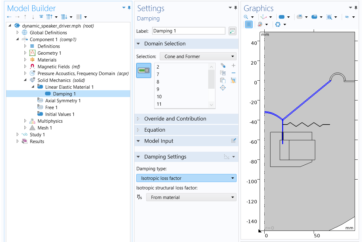The COMSOL Multiphysics UI showing the Modeling Builder with the Damping feature selected, the Settings window with Isotropic loss factor selected as the damping type, and the cone and former highlighted in the Graphics window. An Isotropic loss factor damping model is used to include mechanical loss in the cone and former.

Next, add a second Damping subfeature to the Solid Mechanics > Linear Elastic Material 1 node, select Spider in the Domain Selection section. In the Damping Settings section, choose Rayleigh damping for Damping type and enter 0.14/omega0 for Stiffness damping parameter.

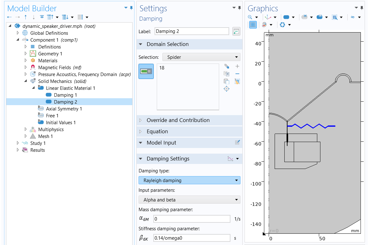The COMSOL Multiphysics UI showing the Modeling Builder with a second Damping feature selected, the Settings window with Rayleigh damping set as the damping type, and the spider highlighted in the Graphics window. A Rayleigh damping damping model is used to include mechanical loss in the spider.

Lastly, add a third Damping subfeature to the Solid Mechanics > Linear Elastic Material 1 node, select Surround in the Domain Selection section. In the Damping Settings section, choose Rayleigh damping for Damping type and enter 0.46/omega0 for Stiffness damping parameter.

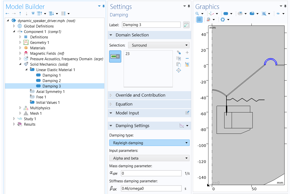The COMSOL Multiphysics UI showing the Modeling Builder with a third Damping feature selected, the Settings window with Rayleigh damping set as the damping type, and the surround highlighted in the Graphics window. A Rayleigh damping damping model is used to include mechanical loss in the surround.

Mechanical Constraints

Any part of the geometry that is fixed or restricted to move in certain directions needs to be modeled. In this example, the end edges of the spider and surround are fixed, as seen below.

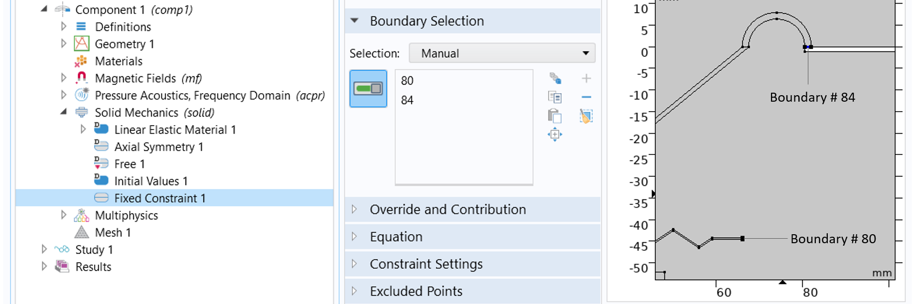A Fixed Constraint boundary feature is applied to the end edges of the spider and surround.

Defining the Materials

You can define the material properties right after the geometry is created, which is straightforward for a single physics model that uses only one material model. However, for a multiphysics model or when multiple material models are used, different material properties are required for different physical domains. In this case, it is more convenient to define material properties after all physics are set up and all material models are specified.

In this exercise, we use the Import Materials From feature to import the eight materials from the dynamic_speaker_driver.mph file via following the steps:

1. Right-click the Materials node and select Import Materials From.
2. Browse to the folder where the file named dynamic_speaker_driver.mph is saved and click Open.
3. Select all materials (press down the Shift key when selecting) and click OK. This adds all the materials from the dynamic_speaker_driver.mph file.
4. Make domain selection for each material. Select Air Domains for Air (mat1), Pole Piece and Top Plate for Soft Iron (With Losses) (mat2), Cone for Composite (mat3), Spider for Cloth (mat4), Surround for Foam (mat5), Coil for Coil (mat6), Former for Glass Fiber (mat7), and Magnet for Generic Ferrite (mat8).

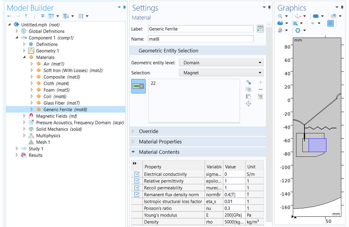Make a domain selection for each material to apply the required material properties for the analysis.

Meshing

For computing the electric impedance, the mesh needs to resolve the induced eddy currents in the pole piece as well as the top plate. In order to obtain accurate results, it is recommended to use at least 1, but preferably 2 quadratic elements to resolve the skin depth.

Iron has a conductivity of 1.12e7 S/m and a peak relative permeability of 1200, so the skin depth in the iron domains will not go below 0.05 mm for a maximum study frequency of 8 kHz. In practice, a majority of the induced currents will run in areas of the pole piece where the biased relative permeability is far less than 1200, resulting in greater skin depth. For this model, it is thus suitable to use a 0.5-mm-sized mesh along the iron surfaces lying closest to the voice coil.

In addition, the air domain and the thin moving structures need to be well resolved for the acoustic–structure interaction. In general, you need 5–6 second-order mesh elements for each wavelength in order to resolve the waves. (See Meshing (Resolving the Waves) in the Acoustics Module User’s Guide for more details.) In this model we use 5 elements per wavelength in the acoustic domains.

For this exercise, we use the same meshing sequence as in the attached dynamic_speaker_driver.mph tutorial model, as shown in the image below.

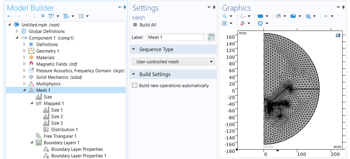The mesh used in this exercise.

Here are some notes about the mesh:

1. At the main Size node, use lam0/5 to customize the maximum element size. This ensures that the mesh is able to resolve the wavelength up to the highest study frequency.
2. A mapped mesh is used to discretize the thin domains, including the cone, the surround, the spider, the former, the coil, and the narrow air gaps where the Narrow Region Acoustics feature is applied. Three Size subnodes are used to control the mesh resolution in different domains, and a Distribution feature is used to specify the number of mesh elements in the thickness direction.
3. A free triangular mesh is used for the rest of the domains, the resolution of which is controlled by the main Size node.
4. A Boundary Layers feature is used to apply thin boundary layer meshes to specific boundaries as necessary. The first Boundary Layer Properties subnode is for creating boundary layer meshes to the boundaries in the soft iron domains to resolve the induced eddy currents in the pole piece and the top plate, as seen in the left image in the figure below. The second Boundary Layer Properties subnode is for creating a single boundary layer mesh to the exterior field boundary of the top air domain to enhance the precision of the exterior field calculation, as shown in the right image in the figure below. The Helmholtz-Kirchhoff integral used for the exterior field calculation involves evaluating the normal gradient of acoustic pressure and therefore a finer mesh resolution in the normal direction of the evaluation surface gives more accurate exterior field solution.

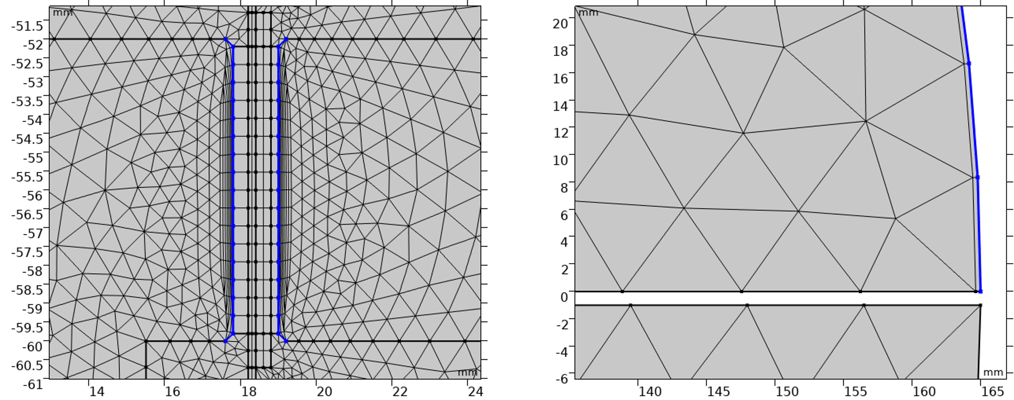Boundary layer meshes are used for finer mesh resolution in the normal direction of the highlighted surfaces to resolve the induced eddy currents in the pole piece and top plate (left) and to enhance the precision of the exterior field calculation (right).

Make sure the Smooth transition to interior mesh check box is cleared at the Transition section of the Boundary Layers 1 settings window so that the boundary layer meshes do not affect the interior mesh that has been generated previously.

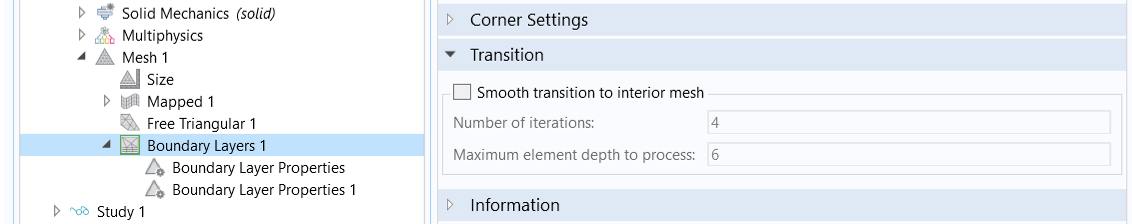Clear the _Smooth transition to interior mesh_ check box so not to allow the boundary layer meshes to affect the interior mesh generated previously.

The Study Setup

The previously added study includes two study steps. For the first Stationary study step, make sure only the check box for the Magnetic Fields physics interface is selected, as shown in the image below.

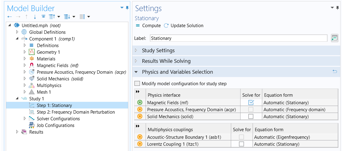The Stationary study step solves for only the Magnetic Fields physics interface.

The second Frequency Domain Perturbation study step solves for all the physics interfaces with all the couplings. The study frequencies include a few frequency points below 10 Hz and ISO preferred frequencies between 10 Hz and 8 kHz. To specify the frequencies in the Frequencies text field in the Study Settings section, follow these steps:

1. Type range(1,1,9).
2. Click Range.
3. In the Range dialog box, choose ISO preferred frequencies from the Entry method list.
4. In the Start frequency text field, type 10.
5. In the Stop frequency text field, type fmax.
6. From the Interval list, choose 1/12 octave.
7. Click Add.

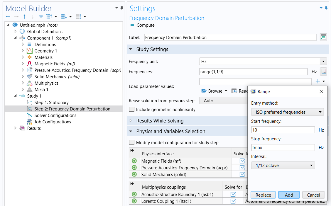The Frequency Domain Perturbation study step solves for all physics interfaces with all couplings.

We can now click Compute to solve the model. The computation time is about one and half minutes.

The Results

After solving the model, several plots are generated automatically that show the results for the magnetic flux density norm, mf.normB, in the magnetic fields domains; the total acoustic pressure, acpr.p_t, in the air domains; and the peak value of Von Mises stress, solid.mises_peak, in the solid domains.

Each step in the study creates its own dataset. Study 1/Solution Store 1 (sol2) contains the stationary solution and Study 1/Solution 1 (sol1) the frequency-domain perturbation. The default plots use the Study 1/Solution 1 (sol1) dataset to evaluate the harmonic perturbation solution. For 2D axisymmetric models, Revolution 2D datasets are automatically generated that allows visualizing the 2D solution in 3D. You have the option to view the static, harmonic perturbation, or total instantaneous solution. Let's take a look at some results.

The static magnetic field in and around the magnetic motor is depicted in the image below. The maximum field in the air arises in the gap between the pole piece and the top plate (the magnetic gap where the voice coil is located).

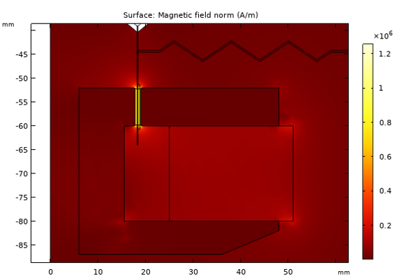
The static magnetic field in and around the magnetic motor.

The iron in the pole piece and the top plate is modeled as a nonlinear magnetic material, with the relationship between the and fields described by interpolation from measured data. The figure below shows the local effective relative permeability . The plot shows that the iron is close to saturation in the center of the pole piece but remains in the linear regime above and below the magnet.

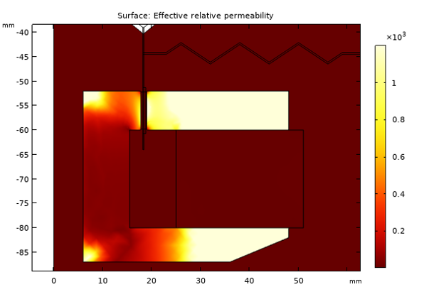
The local relative permeability in the pole piece and top plate when subjected to the field from the magnet.

The image below shows the induced currents at a frequency of 50 Hz and 1000 Hz. With increasing frequency, it is evident that the so-called skin depth decreases as expected.

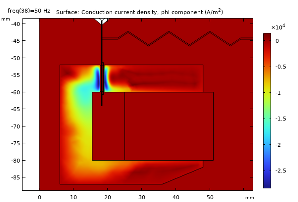
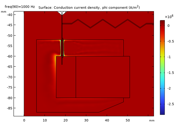
Induced currents in the pole piece and top plate at 50 Hz (top) and 1000 Hz (bottom).

The image below shows the total acoustic pressure and displacement distribution at 8000 Hz in 3D.

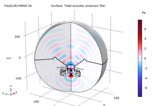
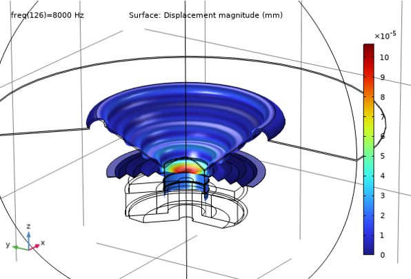
Total acoustic pressure (top) and displacement distribution (bottom) at 8000 Hz.

The total electric impedance, defined as Z = V0/I, is depicted in the figure below (absolute, real, and imaginary parts are plotted). The features of this plot are very characteristic of loudspeaker drivers. The peak at approximately 50 Hz coincides with the mechanical resonance; at this frequency, the reactive part of the impedance switches the sign from inductive to capacitive. In most of the operational range, the impedance is largely resistive. Between 100 Hz and 1 kHz, it varies only between 6.3 Ω and 10.4 Ω. These are typical values for speakers with a nominal impedance of 6.3 Ω, as the nominal impedance is usually taken to represent a mean value over the usable frequency range, which for this driver extends between below 100 Hz and above 1 kHz. The impedance of the speaker as the frequency goes to 0 Hz is 5.6 Ω, which gives the value for the DC resistance. At frequencies higher than 1 kHz, the impedance continues to increase as the inductance of the voice coil starts playing a more important part.

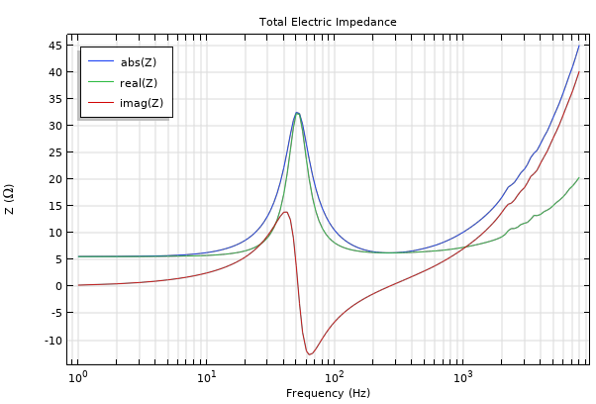
Electric impedance (Ω) of the loudspeaker as a function of frequency (Hz).

The figure below presents the loudspeaker’s sensitivity, depicted both in 1/3 octave bands and as a continuous curve. The plot is realized using the specialized Octave Band plot available in the Acoustics Module. The loudspeaker sensitivity is measured as the on-axis sound pressure level (dB) at a distance of 1 m from the unit. The pressure is evaluated using an input signal of 3.55 V, or 2.51 V RMS, which corresponds to a power of 1 W at 6.3 Ω nominal impedance.

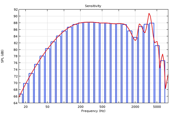
Loudspeaker sensitivity, measured as the on-axis sound pressure level (dB) at a distance of 1 m from the unit.

Lastly, the figure below shows a directivity plot of the spatial speaker response. This is created using the dedicated Directivity plot available with the Acoustics Module. The plot shows a contour representation of the spatial response (measured on a half-sphere in front of the speaker) versus the frequency. The plot is normalized with respect to the level at 0^°.

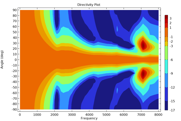
Directivity plot of the spatial speaker response.

See the attached dynamic_speaker_driver.mph file for how these plots are generated.

Additional Learning Resource

The Loudspeaker Driver — Frequency-Domain Analysis tutorial in the Application Gallery provides documentation with step-by-step instructions on how to set up the model. It solves the same problem as the exercise we did here, the only difference being that it uses the Perfectly Matched Layer feature instead of the Perfectly Matched Boundary.